15 The DNA Double Helix

Secondary structure of DNA: The Double Helix

DNA was first identified by Friedrich Miescher in 1869. However, it was not until the 1940s that DNA was accepted as the genetic material based on the evidence shown by experiments carried out by Oswald Avery and his colleagues. Avery’s experiments are discussed in the textbook.

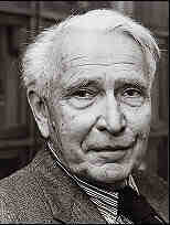
Even then, there still weren’t many scientists studying DNA, and one of them was Erwin Chargaff, in New York (Figure 15.1). He carefully analyzed the composition of DNA and found that the amount of G base in DNA was always nearly the same as the amount of C and the amount of A was always nearly the same as the amount of T. However, the amount of A or T could be quite a lot more, or quite a lot less, than the amount of G or C, depending on the organism that was the source of the DNA sample. We call these relationships “Chargaff’s Rules”: A=T and G=C. Chargaff; however, didn’t grasp the full implications of his discovery.

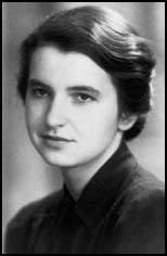
The race to the Double Helix: The race to figure out the structure of DNA is one of the most exciting and important events in scientific history. After the news spread about Avery’s work, a lot of scientists started working on DNA. Rosalind Franklin, at King’s College in London England, tried applying the methods of X-ray crystallography to study DNA. This was before Kendrew had solved the structure of myoglobin (the first protein to be solved by X-ray), so Franklin’s plan was ambitious, to say the least. In the early 1950s, she made a major contribution to the study of DNA.

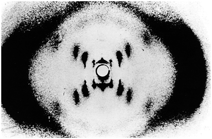
Franklin obtained the first useful X-ray diffraction images of DNA. Franklin’s most famous picture of DNA is the celebrated “photo 51” (Figure 15.3). Most of the early attempts to obtain X-ray pictures of DNA just gave smudges that could not be interpreted. But Franklin persisted, and, by preparing DNA fibres under just the right conditions of hydration, she obtained the blurry but informative “photo 51”. It does not give us high-resolution atomic-level in detail, but it does contain a lot of information about the average structure of the components of the DNA molecule. It showed that the DNA molecules are helical with two periodicities along its long axis: a primary periodicity of 3.4 Å and a secondary one of 34 Å. We won’t discuss how these patterns are interpreted, but there is a nice and understandable presentation available on the web: www.pbs.org/wgbh/nova/photo51/

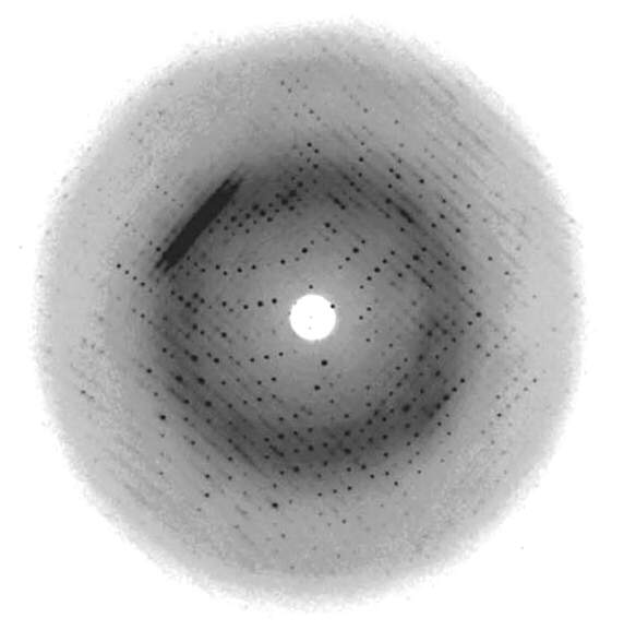
Many years later (1970s), DNA technology had advanced to the point that scientists could synthesize small (a few dozen base pairs) oligonucleotides of defined sequence. These smaller DNA molecules do form well-ordered crystals, and they give “spot” diffraction patterns such as the one shown in Figure 15.4 (Han et al., Acta Cryst. D 56, 104-105, 2000). Those studies provided a great deal of specialized insight into DNA structures (including some unusual structures, such as “zig-zag” or “Z-DNA”, but we won’t discuss those structures in this course), and they showed conclusively that Watson and Crick’s Double Helix model, based on Franklin’s photo 51, was fundamentally correct.

 

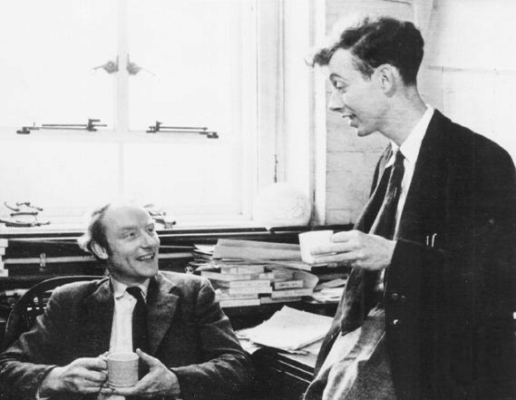
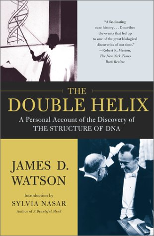
Watson and Crick (Figure 15.5): Francis Crick was a biophysics professor at Cambridge University. James Watson was a young scientist from the USA. (Later, Watson wrote a book called “The Double Helix” (Figure 15.6), in which he tells the story of the discovery. It has an exciting narrative, and you will learn a lot of biochemistry knowledge).

 

Watson and Crick relied on Rosalind Franklin’s “photo 51” to come up with their theoretical model of DNA secondary structure. They realized that the molecule that made the pattern of “photo 51” had to be a helix of some sort. They could even figure out roughly how wide the helix was, and the spacing of the bases along the helix. Watson and Crick tried to build models of DNA and fit them to a helix shape. They were consciously following in the footsteps of Linus Pauling, who had just figured out the protein alpha helix. (In fact, Pauling himself tried to work out the structure of DNA, but the structure he proposed was terrible. Watson and Crick saw right away that it couldn’t possibly be correct).

 

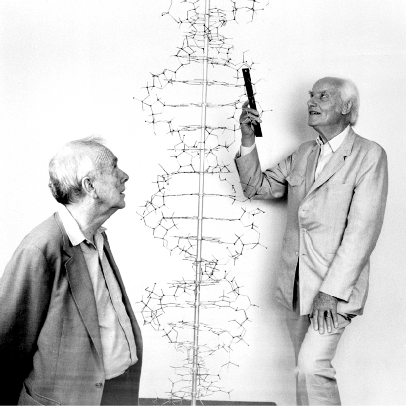
Figure 15.7 shows a reenactment of a famous picture of Watson and Crick standing beside their Double Helix model to mark the 40th anniversary of the discovery of DNA’s structure, done in 1993. Crick was holding a ruler to state that making careful measurements of distances between atoms was really important. Their original one-page paper from 1953 is available at this link (let me know if that link stops working!).

At the start of the paper, they say that the structure “has novel features which are of considerable biological interest.” That’s such an understatement!

 

The breakthrough in understanding DNA structure came when Watson recognized that the purine and pyrimidine bases of DNA can form complementary pairs, linked by sets of hydrogen bonds. Each base pair links a specific purine to a specific pyrimidine: A with T; G with C. One base from each pair resides on one strand, and the other base is on the second strand, which forms a Double Helix.

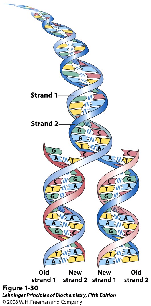
The base-pairing rules mean that each DNA strand encodes the same biological information, in a complementary fashion. That is, if you know the base sequence of one strand, you can write down the sequence of the other strand, just by following the base-pairing rule: A goes with T, and C goes with G. It explained how one DNA molecule could turn into two, with the same sequences: each strand could serve as a “template” (a pattern) for assembly of its partner strand (Figure 15.8). It also explained how a cell or an organism could reproduce through mitosis and meiosis; heredity and genetics. Furthermore, it explained, in principle, how the cell can repair damaged DNA, although nobody thought much about that for a next few years.

 

Watson-Crick base pairs

Knowing the structures of the bases, the Chargaff’s rules, and how H bonds are made, it is easy to figure out how the base pairs form.

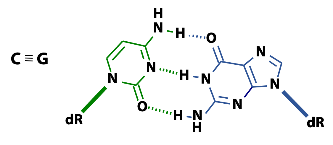
Three hydrogen bonds form between C and G (Figure 15.9). Two hydrogen bonds form between A and T (15.10). The higher the ratio of GC to AT, the more difficult it is to separate two DNA strands.

 

The double helix: Geometry

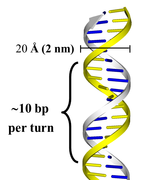
The double helix consists of two antiparallel right handed helices. The base pairs are stacked perpendicular to the helix axis, 3.4 Å apart from each other. Each complete turn of the helix contains ~ 10 base pairs (34 Å). The diameter of the double helix is 20 Å (2 nm) (Figure 15.11).

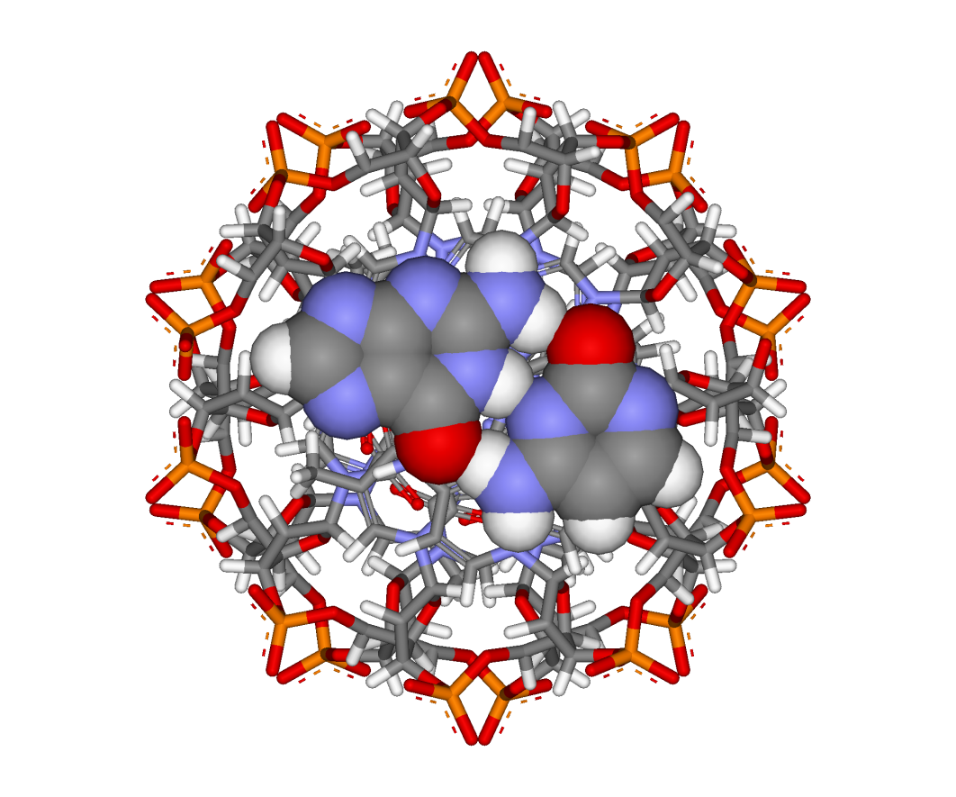
Here are two views: perpendicular to the helix axis (left) and along the helix axis (right). The view in Figure 15.11 corresponds to the original figure in the 1953 paper. In Figure 15.12, you can see clearly how the relatively hydrophobic base pairs are stacked in the core of the double helix perpendicular to the axis, with the hydrophilic sugar-phosphate backbones on the outside, facing the surrounding water.

Figure 15.13 depicts another view perpendicular to the helix axis, showing only a single base pair.

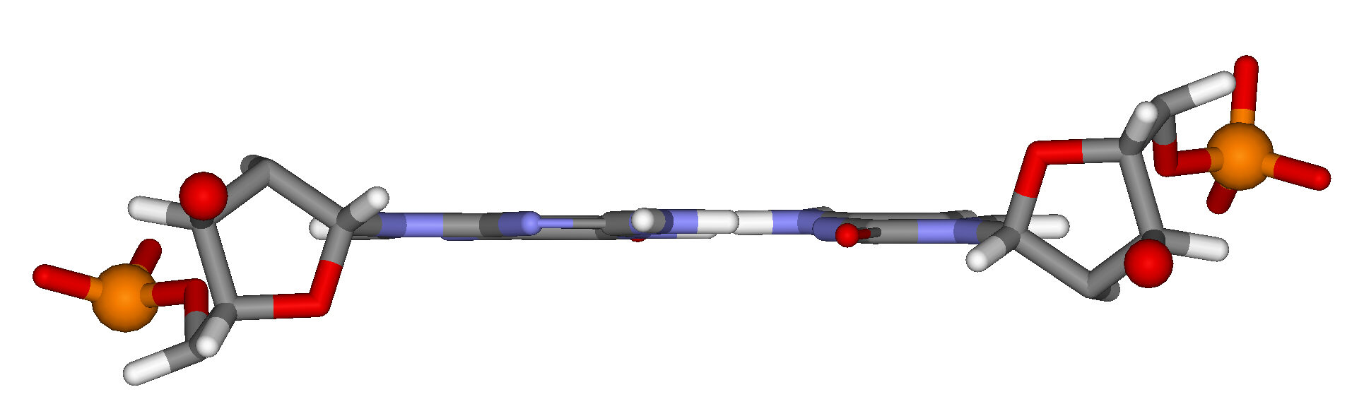
As the 5′ phosphate group and the 3′ oxygen atom of each of the paired nucleotides are shown, you can clearly see that the orientations of the nucleotides and the two strands are antiparallel. (This is analogous to the antiparallel beta structure in protein).

The two strands of the Double Helix are “plectonemically coiled”. This means that they are wrapped around one another, so you can’t pull the two strands apart (unless you start at one end and unwind them).

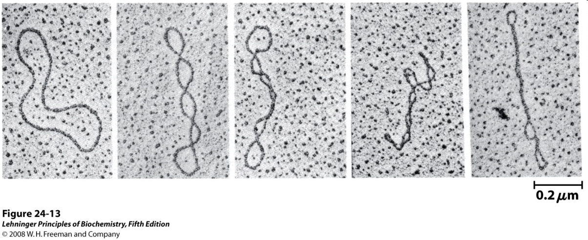
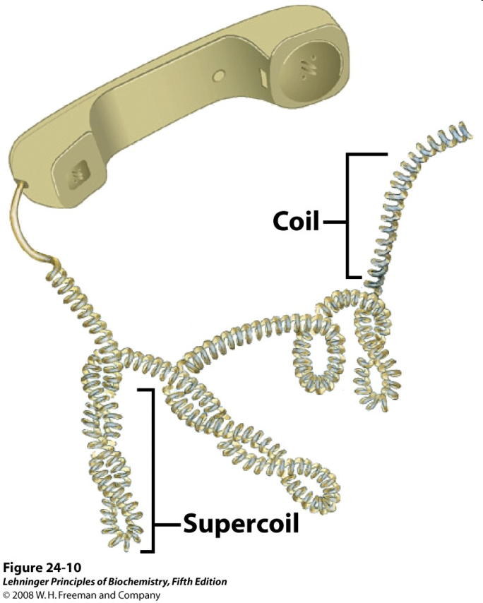
Much like a phone cord (Figure 15.14), DNA undergoes “supercoiling” to give very compact structures (Figure 15.15).

 

 

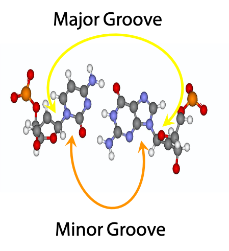
The glycosylic bonds leading to the sugar units of the two base-paired nucleosides are not colinear; they are at an angle. As a result, there is a short angle (minor grove) and a large angle (major groove) between them. When you wind the strands up into the Double Helix, it will result in a large gap between the sugar-phosphate backbones on one side of the helix, and a small gap between the sugar-phosphate backbones on the other side of the helix. (Except that the helix winds around and around, and so do the gaps). These gaps are called the major groove (large gap) and the minor– groove (small gap) (Figure 15.16). As the double helix winds up, major and minor grooves alternate on the surface of the duplex. The image on the right shows a C-G base pair, face on.

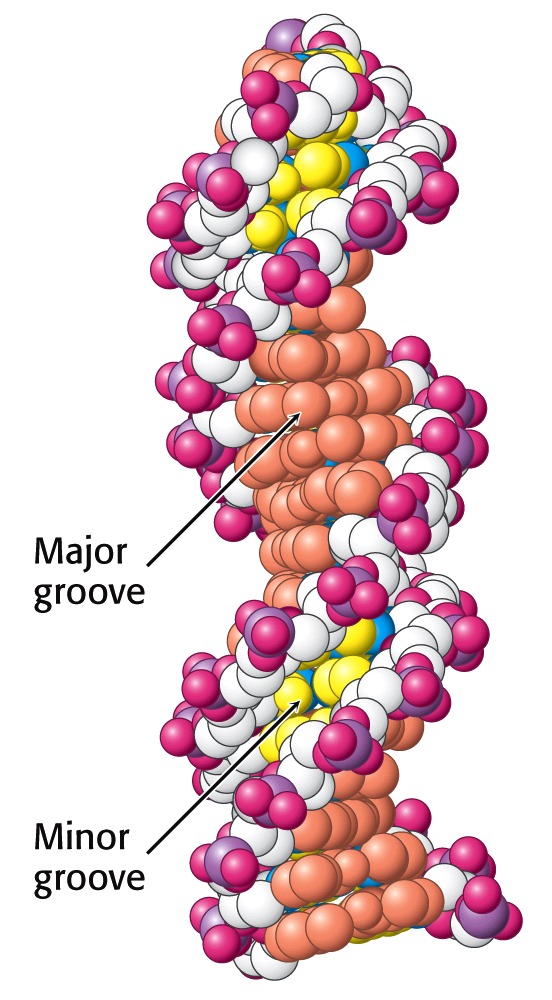
Figure 15.17 shows the major and minor grooves winding around the Double Helix. You can see that the edges of the bases are much more exposed in the major groove than in the minor groove. Each groove is lined by potential hydrogen-bond donor and acceptor atoms of the bases that enable specific interactions with proteins. The larger size of the major groove makes it more accessible for interactions with proteins that recognize specific DNA sequences.

All of this structural biology has important implications for the interactions of proteins with DNA, and, consequently, for gene expression and biological regulation.

 

DNA secondary structure is largely independent of sequence

The side-chains of the amino acids (the sequence) have a huge influence on secondary structure of protein. In contrast, DNA secondary structure is almost independent of its base sequence. (This is an oversimplification; it is not entirely true). That’s because the two kinds of base pairs have very similar shapes and properties.

H-bonds between these base pairs help to hold the DNA Double Helix together, but that’s only part of the story. There is also a big hydrophobic effect: the bases are hydrophobic, so they hide in the core of the helix (like what happens in proteins), and the sugar-phosphate backbone is polar, so it’s on the outside, interacting with water. Moreover, the bases “stack” – they sit almost on top of one another, like a pile of dinner plates in the cafeteria. These van der Waals interactions add up to a large amount of stabilization free energy.

 

The “Central Dogma” of Molecular Biology

By the early 1960s, the work of Francis Crick and others had established the so-called “Central Dogma” of molecular biology, which describes the flow of genetic information (Figure 15.18). (Note that the arrows in the scheme represent flows of information, not chemical transformations.) The gene is comprised of DNA and the double-stranded DNA serves as a “template” (i.e., instruction set) for the synthesis of new DNA molecules. That’s “replication”, which occurs whenever a cell divides. The base sequences of DNA carry the information for the synthesis of proteins: each set of three consecutive DNA bases (a “codon”) specifies one amino acid in the sequence of a protein. DNA also serves as template for synthesis of “messenger RNA” molecules, which carry the same sequence of codons as the DNA. The DNA-templated synthesis of mRNA molecules in the cell is called “transcription” of the gene. In the final stage of information flow, the protein synthesis machinery of the ribosome “reads” the successive triplet mRNA codons and incorporates the corresponding amino acids into polypeptide chains. The “dictionary” for this “translation” process is the genetic code.

That’s as far as we knew, back in the 1960s. This “central dogma” is fundamentally correct, but subsequent discoveries have shown that biology is actually far more complicated. For example, RNA information can flow back into DNA (“reverse transcription”), most of the DNA in eukaryotic cells does not actually encode protein sequences or RNA has turned out to have a myriad of unexpected biological functions, including catalytic activity (“ribozymes”) and the regulation of gene expression (“RNA interference”, the discovery that garnered the Nobel Prize in Medicine for 2006).