Synopsis: The kinetic behaviour of enzymes is described by the Michaelis-Menten equation, and the two characteristic constants associated with this equation, V_max and K_M. Every enzyme has specific values for these constants, which must be measured experimentally. Linear plots like the Lineweaver-Burk plot provide the simplest means of fitting potentially error prone experimental values to the Michaelis-Menten equation.

Inhibitors control enzyme activity by reversibly decreasing the enzyme activity. Different mechanisms of inhibition depend on the relationship between inhibitor and substrate, and can be distinguished by observing how inhibitor affects K_M or V_max of the enzyme.

Competitive inhibition increases K_M with no effect on V_max.

Non-competitive inhibition decreases V_max with no effect on K_M.

Experimental measurement of enzyme kinetic properties

The kinetic properties of enzymes may be characterized by measuring reaction rates for a series of different substrate concentrations. Each rate is measured should be an initial velocity, either by taking the slope of a progress curve ([S] or [P] plotted versus time) at zero time, or by allowing the reaction to proceed for a very brief time and measuring extent of reaction.

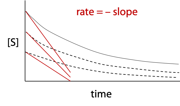
The reaction should be linear over the short time interval.

A different progress curve is obtained for each initial substrate concentration, which is indicated by where the curve starts on the [S] axis (Figure 11.1). A slope is measured for each curve at t = 0. These slopes are the initial rates, v_o used in the Michaelis-Menten plot.

 

The Michaelis Menten hyperbolic plot

Initial rates taken from the progress curves are then plotted as a function of [S]. The graph follows a characteristic hyperbolic shape that matches the Michaelis-Menten equation (right).

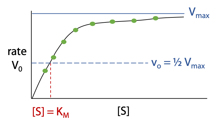
V_max is the limiting maximum rate as [S] tends to infinity (Figure 11.2).

Once V_max has been determined we find the point on the curve where v_o = ½ V_max; the concentration [S] at this point gives the value of K_M.

K_M and V_max tell you about the enzyme’s properties as a catalyst.

V_max indicates catalytic rate when 100% of enzyme is occupied by substrate, higher V_max means faster reaction, better catalyst

V_max is not a true constant – it is only constant if the same amount of enzyme is used for each rate measurement. V_max is proportional to the concentration of enzyme present:

V_max = k₂[E]_total

From V_max, we can calculate the true constant k₂, the rate constant for the catalytic step of the two step enzyme reaction. k₂ (sometimes written as k_cat) is the turnover number of the enzyme (Figure 11.3).

K_M indicates the affinity of the substrate for the enzyme.

• Low K_M means high affinity, the enzyme binds this substrate more strongly
• High K_M means low affinity, the enzyme binds this substrate more weakly

An enzyme that recognizes different substrates will have a different K_M for each substrate. To measure K_M of substrate B, keep [A] high and constant, measure rate as a function of varying [B].

---

Measuring V_max and K_M can be tricky

Unfortunately it’s not as easy as it seems to estimate V_max by inspection of the hyperbolic plot, since the curve keeps creeping up even at very high [S]. Most people underestimate V_max by 10-20% when using this method (Figure 11.4). If the estimate of V_max is bad, the estimate of ½ V_max and K_M is also affected.

Real experimental data also tends to scatter off the theoretical curve due to measurement errors, making graphing the correct curve even more difficult (Figure 11.5).

Linear plots

Instead, the Michaelis-Menten equation may be rewritten so it plots as a straight line, which is much easier for graphing experimental data. This is known as a linear transformation.

Lineweaver-Burk or double reciprocal plot

Take reciprocals of both sides of the Michaelis-Menten equation and then cancel terms (Figure 11.6).

If we substitute y for 1 / v_o and x for 1 / [S], this is now the standard equation for a straight line, with slope = K_M / V_max, and y intercept = 1 / V_max.

A straight-line plot is much preferred over a curve, particularly when the data is slightly scattered due to experimental error. Slopes and intercepts are relatively easily obtained from a straight-line graph. The result is known as the Lineweaver-Burk plot, or double reciprocal plot (Figure 11.7).

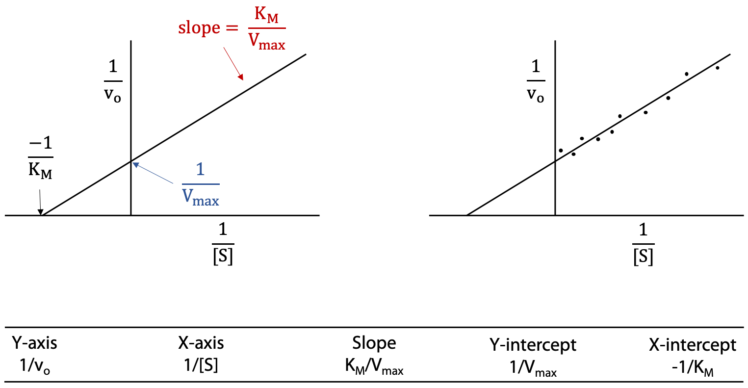
The Lineweaver-Burk plot is usually extrapolated to the negative x-axis. Although there’s no data with negative x values, the negative x-intercept can be used to obtain K_M.

X-intercept = – (Y-intercept) / slope.

A hint for correlating axis labels and intercepts: The y-axis is 1 / v_o, so its intercept is 1 / V_max.The x axis is 1 / [S], so its intercept is – 1 / K_M (the negative sign corrects for the intercept having a negative value). Remember that K_M is a concentration, the concentration [S] that happens to give 50% of maximum rate or 0.5 × V_max.

 

Various substances can act on enzymes to reduce their activity

Inactivation results from a reactive molecule that may form covalent bonds with key amino acids, preventing the enzyme from completing its reaction cycle. Inactivation tends to be irreversible. Essentially, an inactivator reduces the quantity of available enzyme irreversibly and in a stoichiometric manner:

3 µmol enzyme + 2 µmol inactivator leaves 1 µmol enzyme to continue working.

e.g. Disopropylfluorophosphate reacts with acetylcholinesterase irreversibly, blocking transmission of nerve impulses. Many so-called nerve gases act this way and many are halogen-phosphorus compounds.

---

Reversible inhibition results from a substance that binds to an enzyme and limits its capacity to catalyze reaction. The binding is non-covalent and reversible, and if inhibitor is removed, normal activity is restored. The concentration of inhibitor, like substrate, is typically much higher than enzyme concentration.

Enzymes need to be regulated in the course of normal metabolism, i.e. an enzyme that is temporarily not needed is turned off. Reversible inhibition can contribute to regulation, since activity can be restored by removing the inhibitor without having to make new enzyme. Enzyme regulation and its consequences are major themes of BIOC*3560.

Many of the substances that we use as drugs acting by inhibiting a key enzyme in the body. For example, acetylsalicylic acid (ASA or aspirin) inhibits an enzyme called cyclooxygenase, which is responsible for making prostaglandins that stimulate the inflammatory response. When ASA inhibits cyclooxygenase, less prostaglandin is made and inflammation is kept under control. Finding and analyzing properties of enzyme inhibitors is an important aspect of pharmaceutical research.

There are several reversible inhibition mechanisms, distinguished by the relationship between inhibitor and the substrate of the enzyme.

1. Competitive inhibition: the enzyme either binds substrate or binds inhibitor, but not both. In other words, the substrate and inhibitor compete for occupation of the enzyme molecule.
2. Non-competitive inhibition: inhibitor can bind to enzyme whether substrate is also bound or not, i.e. substrate binding has no effect on inhibition.
3. Uncompetitive inhibition: opposite to competitive, the inhibitor can only bind to the ES complex if substrate bind first. This mode may occur with two-substrate enzymes. We won’t be discussing this mode other than to mention it here.
4. Mixed inhibition: is the combination of non-competitive with either of the other mechanisms. The true non-competitive inhibition is rare. In fact, most cases are actually mixed inhibition that closely approximates the non-competitive case.

1. Competitive inhibition:

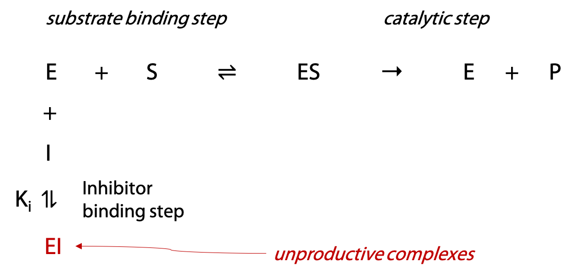
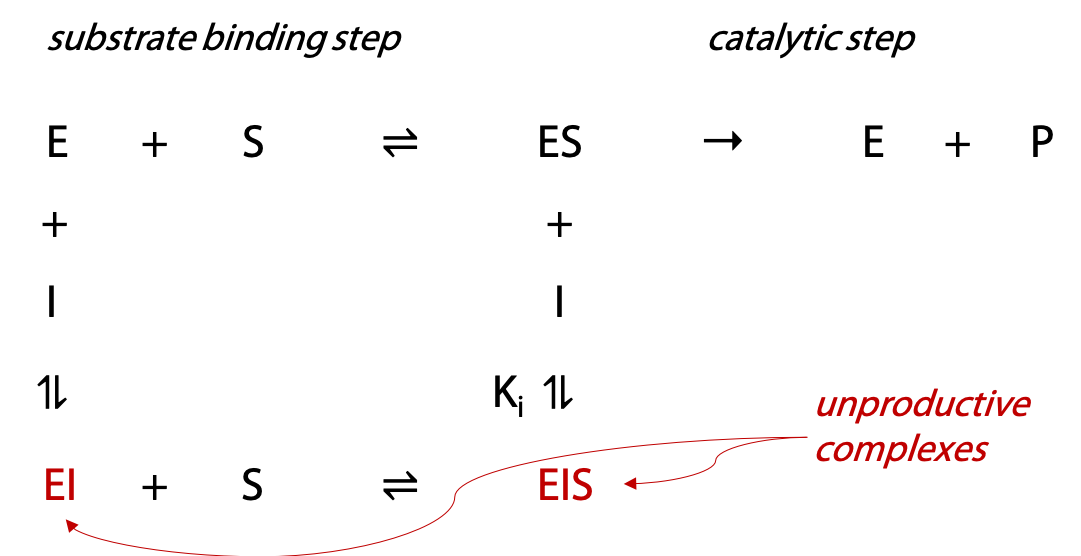
A competitive inhibitor I can only bind to the unoccupied enzyme E, not to the ES complex (Figure 11.8). The quantity of complex EI that forms is governed by the equilibrium constant K_i, known as the inhibition constant. If more EI forms, less enzyme is available to form productive ES complex.

However, since inhibitor I can’t bind to ES, very high substrate concentrations can overcome the inhibitor by forcing the substrate binding equilibrium in the direction of ES, and this brings the enzyme up to its normal V_max. Hence the term competitive to describe this inhibition.

Michaelis Menten hyperbolic plot: shows the rate v_o of the enyme reaction with a constant concentration [I] of inhibitor as [S] is varied (Figure 11.9).

The rate rises more gradually when inhibitor is present, but eventually reaches approaches the normal V_max when [S] is very high.

If inhibitor concentration [I] is set equal to K_i, this causes the K_M‘ observed to be doubled relative to uninhibited enzyme.

Characteristics of a competitive inhibitor: V_max is unchanged, observed K_M‘ increases.

• In the presence of inhibitor at concentration [I],
• Remember higher K_M implies that the enzyme binds its substrate with lower affinity. i.e. a higher concentration of [S] is needed before the enzyme can reach 50% of V_max.
• K_i is equal to the concentration of inhibitor that doubles the observed K_M of the enzyme. If we set the inhibitor concentration [I] = K_i, then . The term   is the inhibition factor, and appears in all inhibition equations.

 

The change in K_M is detected by plotting the data in one of the linear forms, e.g. in the Lineweaver Burk Plot (Figure 11.10) —

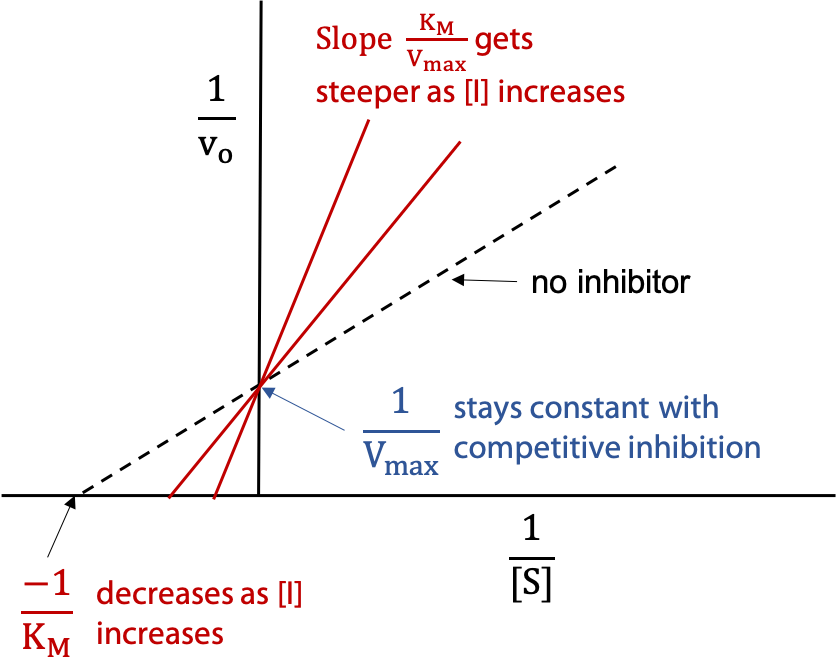
The dashed line represents the activity of the normal uninhibited enzyme, and then the experiment is repeated with a series of different concentrations of I. The other two lines show the effect increasing [I] .

Each line shows the behaviour of the enzyme for a given value of [I]. The higher concentration of inhibitor gives a steeper slope to the line. The series of lines pivot on the y intercept, since V_max is not changed for competitive inhibition. The X-intercept becomes smaller as [I] increases, since K_M increases for competitive inhibition.

To measure K_i, one finds the inhibitor concentration [I] that doubles the observed K_M‘. This is represented by the middle line in the figure (x-intercept halved means K_M‘ was doubled.).

2. Non-competitive inhibition:

A non-competitive inhibitor I can bind both to unoccupied enzyme E, and to ES complex (Figure 11.11). The EI complex can bind S, but EIS is unable to proceed to give products.

The quantity of complexes EI and EIS that form are governed by the equilibrium constant K_i. If more EI or EIS forms, less enzyme is available to form productive ES complex. Since I can also bind to ES, high substrate concentrations do not overcome the inhibitor. Hence the term non-competitive to describe this inhibition. True non-competitive inhibition requires K_i to be the same at both stages (this is rare). If the K_i for I binding to empty E is not the same as for I binding to occupied ES, mixed inhibition will be observed.

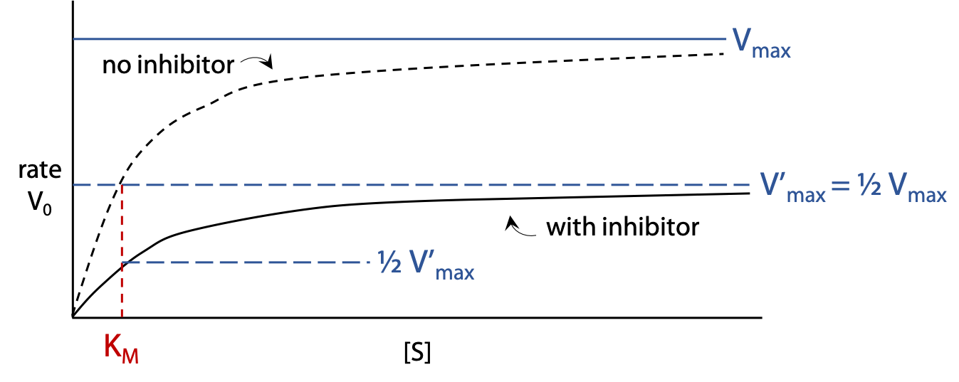
Michaelis Menten hyperbolic plot (Figure 11.12): shows the rate v_o of the enzyme reaction with a constant concentration [I] of inhibitor as [S] is varied. The rate rises more gradually when inhibitor is present, and levels off at a lower V’_max.

If inhibitor concentration [I] is set equal to K_i, this causes the V’_max observed to be halved relative to uninhibited enzyme.

Characteristics of a non-competitive inhibitor: V’_max decreases, K_M is unchanged.

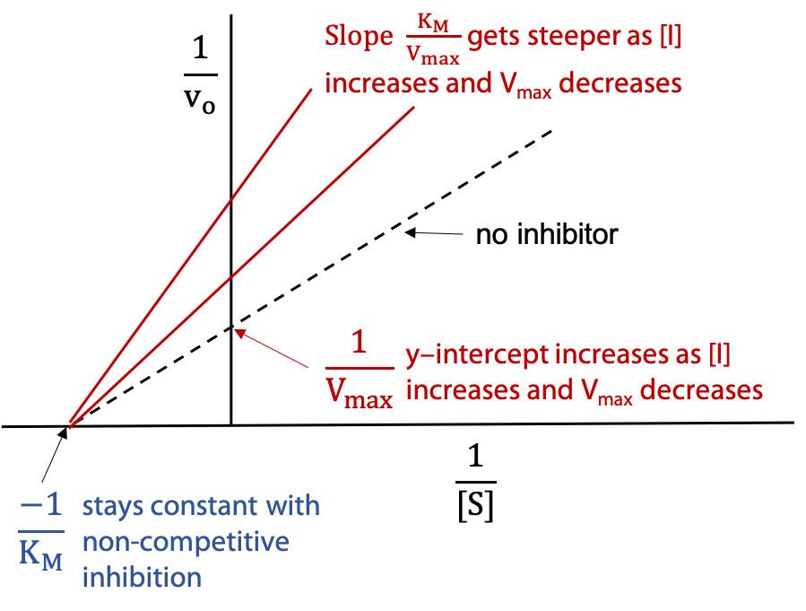
Lineweaver-Burk Plot (Figure 11.13):

The dashed line represents the activity of the uninhibited enzyme. The other two lines show the effect of added inhibitor I. The series of lines pivot on the -ve x-intercept, since K_M is unchanged for non-competitive inhibition. Y-intercept and slope increase due to the reciprocal dependence on V’_max, which decreases. To measure K_i, one finds the inhibitor concentration [I] that halves the observed V’_max.

3. Mixed inhibition

Mixed inhibition is indicated by decrease in V_max coupled to increase in K_M. If the change in V_max is large and the change in K_M‘ is small, then it is a reasonable approximation (and mathematically much simpler) to treat the case as non-competitive.