13 Quality Control During Construction
13.1 Quality Concerns in Construction
Defects or failures in constructed facilities can result in very large costs. Even with minor defects, rework (re-construction) may be required, and facility operations may be impaired. Increased costs and delays are the result. Hwang et al studied 359 construction projects to analyze the sources of rework. Its measured impact typically adds up to 5% of the total project cost, and experienced project managers estimate the real percentage is often much higher. Contrast that with typical profit margins of only a few percent of total project cost. Good project managers try to ensure that the job is done right the first time. Quality control is essential in that regard.
As with cost control, the most important decisions regarding the quality of a completed facility are made during the design and planning stages rather than during construction. It is during these preliminary stages that component configurations, material specifications and functional performance are decided. Quality control during construction consists largely of insuring conformance to these original design and planning decisions.
While conformance to existing design decisions is the primary focus of quality control, there are exceptions to this rule. First, unforeseen circumstances, incorrect design decisions or changes desired by an owner in the facility function may require re-evaluation of design decisions during the course of construction. While these changes may be motivated by the concern for quality, they represent occasions for re-design with all the attendant objectives and constraints.
As a second case, and it is not the focus of this chapter, some designs rely upon informed and appropriate decision making during the construction process itself. In many ways, the submittals process in building construction reflects this fact. The owner’s architect and engineer will specify equipment (such as cooling equipment, window systems, etc.) and materials (such as floor finishes, hardware and furnishings) in general terms of performance and quality. Just before and during construction, the contractor will submit specific product options with their performance specifications and prices to the owner or their AE firm for approval. This leads to the classic conpcept of the quality-cost-schedule trade-off triangle shared in many construction project management text books, however “quality” in this context is defined as the architectural massing and design, richness and finish of materials, craftsmanship, landscaping and other aspects of the building. In this chapter, we are focused on conformance to design intent.
With the attention to conformance as the measure of quality during the construction process, the specification of quality requirements in the design and contract documentation becomes extremely important. Quality requirements should be clear and verifiable, so that all parties in the project can understand the requirements for conformance. Much of the discussion in this chapter relates to the development and the implications of different quality requirements for construction as well as the issues associated with ensuring conformance.
13.2 Organizing for Quality
In large organizations, departments dedicated to quality assurance might assign specific individuals to assume responsibility for this function on particular projects. For smaller projects, the project manager or an assistant might assume this and other responsibilities. In either case, ensuring quality construction is a concern of the project manager in overall charge of the project in addition to the concerns of personnel, cost, time, safety, health and other management issues.
Inspectors and quality assurance personnel will be involved in a project to represent a variety of different organizations. Each of the parties directly concerned with the project may have their own quality inspectors, including the owner, the engineer/architect, and the various constructor firms. These inspectors may be contractors from specialized quality assurance organizations. In addition to on-site inspections, samples of materials will commonly be tested by specialized laboratories to ensure compliance. Inspectors to ensure compliance with regulatory requirements will also be involved. Common examples are inspectors for the local government’s building department, for environmental agencies, and for occupational health and safety agencies.
While the multitude of participants involved in the construction process require the services of inspectors, it cannot be emphasized too strongly that inspectors are only a formal check on quality control. Quality control should be a primary objective for all the members of a project team. Managers should take responsibility for maintaining and improving quality control. Employee participation in quality control should be sought and rewarded, including the introduction of new ideas. Most important of all, quality improvement can serve as a catalyst for improved productivity. By suggesting new work methods, by avoiding rework, and by avoiding long term problems, good quality control can pay for itself. Owners should promote good quality control and seek out contractors who maintain such standards.
In addition to the various organizational bodies involved in quality control, issues of quality control arise in virtually all the functional areas of construction activities. For example, insuring accurate and useful information is an important part of maintaining quality performance. Other aspects of quality control include document control (including changes during the construction process), procurement, field inspection and testing, and final checkout of the facility.
13.3 Work and Material Specifications
Specifications of work quality are an important feature of facility designs. Specifications of required quality and components represent part of the necessary documentation to describe a facility. Typically, this documentation includes any special provisions of the facility design as well as references to generally accepted specifications to be used during construction.
General specifications of work quality are available in numerous fields and are issued in publications of organizations such as the American Society for Testing and Materials (ASTM), the American National Standards Institute (ANSI), the American Institute of Steel Construction (AISC), or the Construction Specifications Institute (CSI). The National Institute for Standards and Technology (NIST) plays a crucial role though its various laboratories, such as the National Voluntary Laboratory Accreditation Program (NVLAP). Distinct specifications are formalized for particular types of construction activities, such as welding standards issued by the American Welding Society, or for particular facility types, such as the Standard Specifications for Highway Bridges issued by the American Association of State Highway and Transportation Officials (AASHTO). These general specifications must be modified to reflect local conditions, policies, available materials, local regulations and other special circumstances.
In Canada, various provincial and federal ministries will impose construction, environmental and design standards. An example is the Ministry of Transportation of Ontario (MTO). Since Canadians participate in many US standards organizations, such as AASHTO, some of their specifications will be adapted from those organizations for Canadian conditions. A lead issuer of specifications in Canada that also influences US specifications is the CSA Group. According to their infrastructure web site:
“CSA Group is a trusted leader in standards development for the construction industry. For over 100 years, CSA Group has produced standards behind the design and construction of buildings and infrastructure including structural design, systems and resiliency, and manufacture and certification of construction products. Today we have more than 250 standards – many referenced in legislation and construction specifications – that help safeguard human life and contribute to the progressive improvement of the construction industry.”
Construction contract specifications normally consist of a series of instructions or prohibitions for specific operations. For example, the following passage illustrates a typical specification, in this case for excavation for structures:
“Conform to elevations and dimensions shown on plan within a tolerance of plus or minus 0.10 foot, and extending a sufficient distance from footings and foundations to permit placing and removal of concrete formwork, installation of services, other construction, and for inspection. In excavating for footings and foundations, take care not to disturb bottom of excavation. Excavate by hand to final grade just before concrete reinforcement is placed. Trim bottoms to required lines and grades to leave solid base to receive concrete.”
This set of specifications requires judgment in application since some items are not precisely specified. For example, excavation must extend a “sufficient” distance to permit inspection and other activities. Obviously, the term “sufficient” in this case may be subject to varying interpretations. In contrast, a specification that tolerances are within plus or minus a tenth of a foot is subject to direct measurement. However, specific requirements of the facility or characteristics of the site may make the standard tolerance of a tenth of a foot inappropriate. Writing specifications typically requires a trade-off between assuming reasonable behavior on the part of all the parties concerned in interpreting words such as “sufficient” versus the effort and possible inaccuracy in pre-specifying all operations.
In recent years, performance specifications have been developed and applied for many construction operations. Rather than specifying the required construction process, these specifications refer to the required performance or quality of the finished facility. The exact method by which this performance is obtained is left to the construction contractor. For example, traditional specifications for asphalt pavement specified the composition of the asphalt material, the asphalt temperature during paving, and compacting procedures. In contrast, a performance specification for asphalt details the desired performance of the pavement with respect to impermeability, longitudinal roughness, surface friction, strength, rutting resistance over time, etc. How the desired performance level was attained would be up to the paving contractor. In some cases, the payment for asphalt paving might increase with better quality of asphalt beyond some minimum level of performance, and it might be tied to performance over many years, if a maintenance element is included in the contract.
Example 13-1: Concrete Pavement Strength
Concrete pavements of superior strength result in cost savings by delaying the time at which repairs or re-construction is required. In contrast, concrete of lower quality will necessitate more frequent overlays or other repair procedures. Contract provisions with adjustments to the amount of a contractor’s compensation based on pavement quality have become increasingly common in recognition of the cost savings associated with higher quality construction. Even if a pavement does not meet the “ultimate” design standard, it is still worth using the lower quality pavement and re-surfacing later rather than completely rejecting the pavement. Based on these life cycle cost considerations, a typical pay schedule might be: [1]
| Load Ratio | Pay Factor |
| <0.50 0.50-0.69 0.70-0.89 0.90-1.09 1.10-1.29 1.30-1.49 >1.50 |
Reject 0.70 0.85 1.00 1.05 1.10 1.12 |
In this table, the Load Ratio is the ratio of the actual pavement strength to the desired design strength and the Pay Factor is a fraction by which the total pavement contract amount is multiplied to obtain the appropriate compensation to the contractor. For example, if a contractor achieves concrete strength twenty percent greater than the design specification, then the load ratio is 1.20 and the appropriate pay factor is 1.05, so the contractor receives a five percent bonus. Load factors are computed after tests on the concrete actually used in a pavement. Note that a 70% pay factor exists in this case with even pavement quality only 50% of that originally desired. This high pay factor even with weak concrete strength (and thus radically shortened design life) might exist since much of the cost of pavements are incurred in preparing the pavement foundation. Concrete strengths of less then 50% are cause for complete rejection in this case, however.
13.4 Total Quality Control
Quality control in construction typically involves ensuring compliance with minimum standards of material and workmanship in order to insure the performance of the facility according to the design. These minimum standards are contained in the specifications described in the previous section. For the purpose of ensuring compliance, random samples and statistical methods are commonly used as the basis for accepting or rejecting work completed and batches of materials. Rejection of a batch is based on non-conformance or violation of the relevant design specifications. Procedures for this quality control practice are described in the following sections.
An implicit assumption in these traditional quality control practices is the notion of an acceptable quality level which is an allowable fraction of defective items. Materials obtained from suppliers or work performed by an organization is inspected and passed as acceptable if the estimated defective percentage is within the acceptable quality level. Problems with materials or goods are corrected after delivery of the product.
In contrast to this traditional approach of quality control is the goal of total quality control. In this system, no defective items are allowed anywhere in the construction process. While the zero defects goal can never be permanently obtained, it provides a goal so that an organization is never satisfied with its quality control program even if defects are reduced by substantial amounts year after year. This concept and approach to quality control was first developed in manufacturing firms in Japan and Europe, but it has since spread to many construction companies. The best-known formal certification for quality improvement is the International Organization for Standardization’s ISO 9000 standard. ISO 9000 emphasizes good documentation, quality goals and a series of cycles of planning, implementation and review.
Total quality control is a commitment to quality expressed in all parts of an organization and typically involves many elements. Design reviews to insure safe and effective construction procedures are a major element. Other elements include extensive training for personnel, shifting the responsibility for detecting defects from quality control inspectors to workers, and continually maintaining equipment. Worker involvement in improved quality control is often formalized in quality circles in which groups of workers meet regularly to make suggestions for quality improvement. Material suppliers are also required to insure zero defects in delivered goods. Initially, all materials from a supplier are inspected and batches of goods with any defective items are returned. Suppliers with good records can be certified and not subject to complete inspection subsequently.
The traditional microeconomic view of quality control is that there is an “optimum” proportion of defective items. Trying to achieve greater quality than this optimum would substantially increase costs of inspection and reduce worker productivity. However, many companies have found that commitment to total quality control has substantial economic benefits that had been unappreciated in traditional approaches. Expenses associated with inventory, rework, scrap and warranties were reduced. Worker enthusiasm and commitment improved. Customers often appreciated higher quality work and would pay a premium for good quality. As a result, improved quality control became a competitive advantage.
Of course, total quality control is difficult to apply, particularly in construction. The unique nature of each facility, the variability in the workforce, the multitude of subcontractors and the cost of making necessary investments in education and procedures make programs of total quality control in construction difficult. Nevertheless, a commitment to improved quality even without endorsing the goal of zero defects can pay real dividends to organizations.
Example 13-2: Experience with Quality Circles
Quality circles represent a group of five to fifteen workers who meet on a frequent basis to identify, discuss and solve productivity and quality problems. A circle leader acts as liaison between the workers in the group and upper levels of management. Appearing below are some examples of reported quality circle accomplishments in construction: [2]
-
- On a highway project under construction by Taisei Corporation, it was found that the loss rate of ready-mixed concrete was too high. A quality circle composed of cement masons found out that the most important reason for this was due to an inaccurate checking method. By applying the circle’s recommendations, the loss rate was reduced by 11.4%.
- In a building project by Shimizu Construction Company, may cases of faulty reinforced concrete work were reported. The iron workers quality circle examined their work thoroughly and soon the faulty workmanship disappeared. A 10% increase in productivity was also achieved.
13.5 Quality Control by Statistical Methods
An ideal quality control program might test all materials and work on a particular facility. For example, non-destructive techniques such as x-ray inspection of welds can be used throughout a facility. An on-site inspector can witness the appropriateness and adequacy of construction methods at all times. Even better, individual craftsmen can perform continuing inspection of materials and their own work. Exhaustive or 100% testing of all materials and work by inspectors can be exceedingly expensive, however. In many instances, testing requires the destruction of a material sample, so exhaustive testing is not even possible. As a result, small samples are used to establish the basis of accepting or rejecting a particular work item or shipment of materials. Statistical methods are used to interpret the results of test on a small sample to reach a conclusion concerning the acceptability of an entire lot or batch of materials or work products.
The use of statistics is essential in interpreting the results of testing on a small sample. Without adequate interpretation, small sample testing results can be quite misleading. As an example, suppose that there are ten defective pieces of material in a lot of one hundred. In taking a sample of five pieces, the inspector might not find any defective pieces or might have all sample pieces defective. Drawing a direct inference that none or all pieces in the population are defective on the basis of these samples would be incorrect. Due to this random nature of the sample selection process, testing results can vary substantially. It is only with statistical methods that issues such as the chance of different levels of defective items in the full lot can be fully analyzed from a small sample test.
There are two types of statistical sampling which are commonly used for the purpose of quality control in batches of work or materials:
- The acceptance or rejection of a lot is based on the number of defective (bad) or nondefective (good) items in the sample. This is referred to as sampling by attributes.
- Instead of using defective and nondefective classifications for an item, a quantitative quality measure or the value of a measured variable is used as a quality indicator. This testing procedure is referred to as sampling by variables.
Whatever sampling plan is used in testing, it is always assumed that the samples are representative of the entire population under consideration. Samples are expected to be chosen randomly so that each member of the population is equally likely to be chosen. Convenient sampling plans such as sampling every twentieth piece, choosing a sample every two hours, or picking the top piece on a delivery truck may be adequate to ensure a random sample if pieces are randomly mixed in a stack or in use. However, some convenient sampling plans can be inappropriate. For example, checking only easily accessible joints in a building component is inappropriate since joints that are hard to reach may be more likely to have erection or fabrication problems.
Another assumption implicit in statistical quality control procedures is that the quality of materials or work is expected to vary from one piece to another. This is certainly true in the field of construction. While a designer may assume that all concrete is exactly the same in a building, the variations in material properties, manufacturing, handling, pouring, and temperature during setting ensure that concrete is actually heterogeneous in quality. Reducing such variations to a minimum is one aspect of quality construction. Ensuring that the materials actually placed achieve some minimum quality level with respect to average properties or fraction of defectives is the task of quality control.
13.6 Statistical Quality Control with Sampling by Attributes
Sampling by attributes is a widely applied quality control method. The procedure is intended to determine whether or not a particular group of materials or work products is acceptable. In the literature of statistical quality control, a group of materials or work items to be tested is called a lot or batch. An assumption in the procedure is that each item in a batch can be tested and classified as either acceptable or deficient based upon mutually acceptable testing procedures and acceptance criteria. Each lot is tested to determine if it satisfies a minimum acceptable quality level (AQL) expressed as the maximum percentage of defective items in a lot or process.
In its basic form, sampling by attributes is applied by testing a pre-defined number of sample items from a lot. If the number of defective items is greater than a trigger level, then the lot is rejected as being likely to be of unacceptable quality. Otherwise, the lot is accepted. Developing this type of sampling plan requires consideration of probability, statistics and acceptable risk levels on the part of the supplier and consumer of the lot. Refinements to this basic application procedure are also possible. For example, if the number of defectives is greater than some pre-defined number, then additional sampling may be started rather than immediate rejection of the lot. In many cases, the trigger level is a single defective item in the sample. In the remainder of this section, the mathematical basis for interpreting this type of sampling plan is developed.
More formally, a lot is defined as acceptable if it contains a fraction p1 or less defective items. Similarly, a lot is defined as unacceptable if it contains a fraction p2 or more defective units. Generally, the acceptance fraction is less than or equal to the rejection fraction, p1 ≤ p2, and the two fractions are often equal so that there is no ambiguous range of lot acceptability between p1 and p2. Given a sample size and a trigger level for lot rejection or acceptance, we would like to determine the probabilities that acceptable lots might be incorrectly rejected (termed producer’s risk) or that deficient lots might be incorrectly accepted (termed consumer’s risk).
Consider a lot of finite number N, in which m items are defective (bad) and the remaining (N-m) items are non-defective (good). If a random sample of n items is taken from this lot, then we can determine the probability of having different numbers of defective items in the sample. With a pre-defined acceptable number of defective items, we can then develop the probability of accepting a lot as a function of the sample size, the allowable number of defective items, and the actual fraction of defective items. This derivation appears below.
The number of different samples of size n that can be selected from a finite population N is termed a mathematical combination and is computed as:
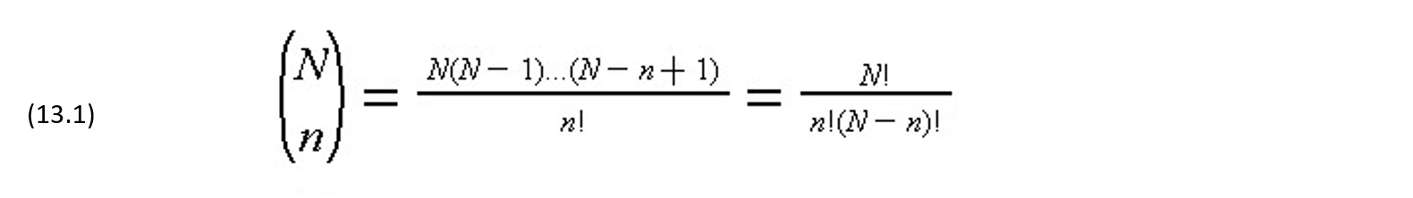
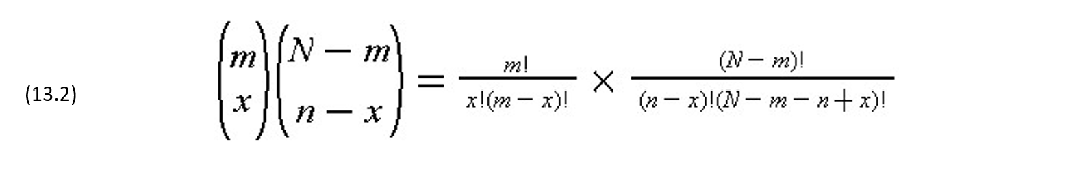
where a factorial, n! is n*(n-1)*(n-2)…(1) and zero factorial (0!) is one by convention. The number of possible samples with exactly x defectives is the combination associated with obtaining x defectives from m possible defective items and n-x good items from N-m good items:
Given these possible numbers of samples, the probability of having exactly x defective items in the sample is given by the ratio as the hypergeometric series:

With this function, we can calculate the probability of obtaining different numbers of defectives in a sample of a given size.
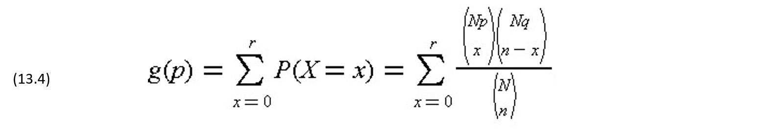
Suppose that the actual fraction of defectives in the lot is p and the actual fraction of nondefectives is q, then p plus q is one, resulting in m = Np, and N – m = Nq. Then, a function g(p) representing the probability of having r or less defective items in a sample of size n is obtained by substituting m and N into Eq. (13.3) and summing over the acceptable defective number of items:
If the number of items in the lot, N, is large in comparison with the sample size n, then the function g(p) can be approximated by the binomial distribution:
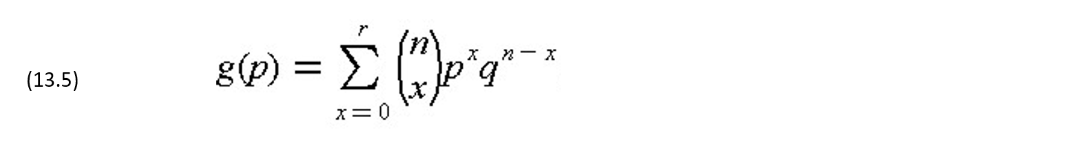
or
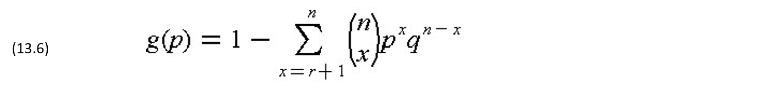
The function g(p) indicates the probability of accepting a lot, given the sample size n and the number of allowable defective items in the sample r. The function g(p) can be represented graphical for each combination of sample size n and number of allowable defective items r, as shown in Figure 13-1. Each curve is referred to as the operating characteristic curve (OC curve) in this graph. For the special case of a single sample (n=1), the function g(p) can be simplified:
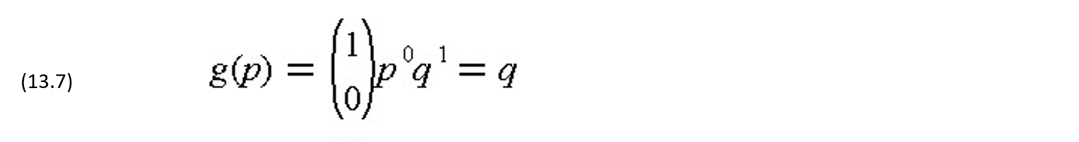
so that the probability of accepting a lot is equal to the fraction of acceptable items in the lot. For example, there is a probability of 0.5 that the lot may be accepted from a single sample test even if fifty percent of the lot is defective.
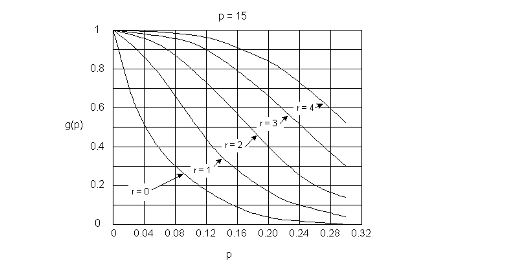
Figure 13-1 Example Operating Characteristic Curves Indicating Probability of Lot Acceptance
For any combination of n and r, we can read off the value of g(p) for a given p from the corresponding OC curve. For example, n = 15 is specified in Figure 13-1. Then, for various values of r, we find:
| r=0 r=0 r=1 r=1 |
p=24% p=4% p=24% p=4% |
g(p) 2% g(p) 54% g(p) 10% g(p) 88% |
The producer’s and consumer’s risk can be related to various points on an operating characteristic curve. Producer’s risk is the chance that otherwise acceptable lots fail the sampling plan (i.e. have more than the allowable number of defective items in the sample) solely due to random fluctuations in the selection of the sample. In contrast, consumer’s risk is the chance that an unacceptable lot is acceptable (i.e. has less than the allowable number of defective items in the sample) due to a better than average quality in the sample. For example, suppose that a sample size of 15 is chosen with a trigger level for rejection of one item. With a four percent acceptable level and a greater than four percent defective fraction, the consumer’s risk is at most eighty-eight percent. In contrast, with a four percent acceptable level and a four percent defective fraction, the producer’s risk is at most 1 – 0.88 = 0.12 or twelve percent.
In specifying the sampling plan implicit in the operating characteristic curve, the supplier and consumer of materials or work must agree on the levels of risk acceptable to themselves. If the lot is of acceptable quality, the supplier would like to minimize the chance or risk that a lot is rejected solely on the basis of a lower-than-average quality sample. Similarly, the consumer would like to minimize the risk of accepting under the sampling plan a deficient lot. In addition, both parties presumably would like to minimize the costs and delays associated with testing. Devising an acceptable sampling plan requires trade off the objectives of risk minimization among the parties involved and the cost of testing.
Example 13-3: Acceptance probability calculation
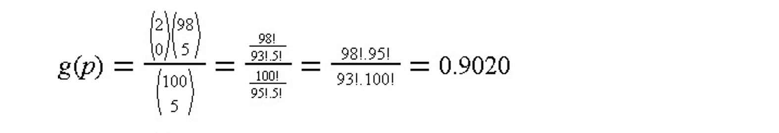
Suppose that the sample size is five (n=5) from a lot of one hundred items (N=100). The lot of materials is to be rejected if any of the five samples is defective (r = 0). In this case, the probability of acceptance as a function of the actual number of defective items can be computed by noting that for r = 0, only one term (x = 0) need be considered in Eq. (13.4). Thus, for N = 100 and n = 5:
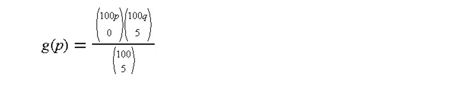
For a two percent defective fraction (p = 0.02), the resulting acceptance value is:
Using the binomial approximation in Eq. (13.5), the comparable calculation would be:
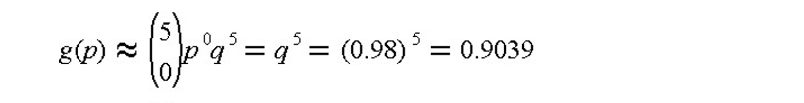
which is a difference of 0.0019, or 0.21 percent from the actual value of 0.9020 found above.
If the acceptable defective proportion was two percent (so p1 = p2 = 0.02), then the chance of an incorrect rejection (or producer’s risk) is 1 – g(0.02) = 1 – 0.9 = 0.1 or ten percent. Note that a prudent producer should insure better than minimum quality products to reduce the probability or chance of rejection under this sampling plan. If the actual proportion of defectives was one percent, then the producer’s risk would be only five percent with this sampling plan.
Example 13-4: Designing a Sampling Plan
Suppose that an owner (or product “consumer” in the terminology of quality control) wishes to have zero defective items in a facility with 5,000 items of a particular kind. What would be the different amounts of consumer’s risk for different sampling plans?
With an acceptable quality level of no defective items (so p1 = 0), the allowable defective items in the sample is zero (so r = 0) in the sampling plan. Using the binomial approximation, the probability of accepting the 5,000 items as a function of the fraction of actual defective items and the sample size is:
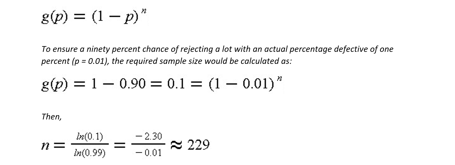
As can be seen, large sample sizes are required to insure relatively large probabilities of zero defective items.
13.7 Statistical Quality Control with Sampling by Variables
As described in the previous section, sampling by attributes is based on a classification of items as good or defective. Many work and material attributes possess continuous properties, such as strength, density or length. With the sampling by attributes procedure, a particular level of a variable quantity must be defined as acceptable quality. More generally, two items classified as good might have quite different strengths or other attributes. Intuitively, it seems reasonable that some “credit” should be provided for exceptionally good items in a sample. Sampling by variables was developed for application to continuously measurable quantities of this type. The procedure uses measured values of an attribute in a sample to determine the overall acceptability of a batch or lot. Sampling by variables has the advantage of using more information from tests since it is based on actual measured values rather than a simple classification. As a result, acceptance sampling by variables can be more efficient than sampling by attributes in the sense that fewer samples are required to obtain a desired level of quality control.
In applying sampling by variables, an acceptable lot quality can be defined with respect to an upper limit U, a lower limit L, or both. With these boundary conditions, an acceptable quality level can be defined as a maximum allowable fraction of defective items, M. In Figure 13-2, the probability distribution of item attribute x is illustrated. With an upper limit U, the fraction of defective items is equal to the area under the distribution function to the right of U (so that x U). This fraction of defective items would be compared to the allowable fraction M to determine the acceptability of a lot. With both a lower and an upper limit on acceptable quality, the fraction defective would be the fraction of items greater than the upper limit or less than the lower limit. Alternatively, the limits could be imposed upon the acceptable average level of the variable
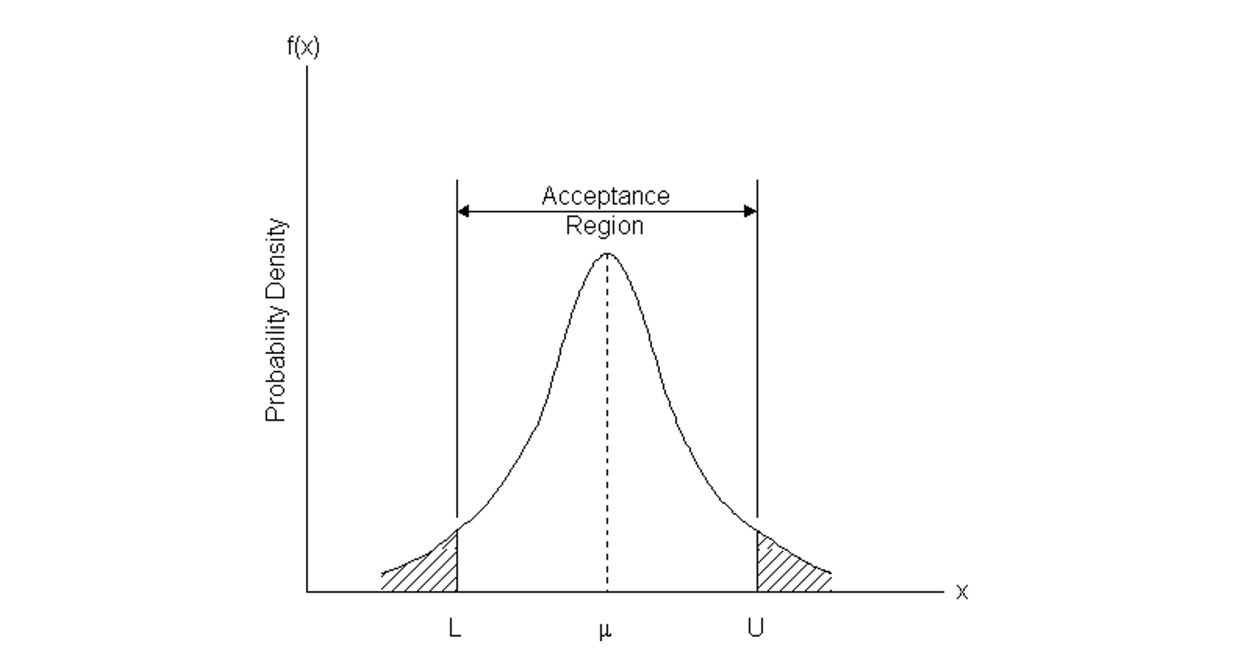
Figure 13-2 Variable Probability Distributions and Acceptance Regions
In sampling by variables, the fraction of defective items is estimated by using measured values from a sample of items. As with sampling by attributes, the procedure assumes a random sample of a give size is obtained from a lot or batch. In the application of sampling by variables plans, the measured characteristic is virtually always assumed to be normally distributed as illustrated in Figure 13-2. The normal distribution is likely to be a reasonably good assumption for many measured characteristics such as material density or degree of soil compaction. The Central Limit Theorem provides a general support for the assumption: if the source of variations is a large number of small and independent random effects, then the resulting distribution of values will approximate the normal distribution. If the distribution of measured values is not likely to be approximately normal, then sampling by attributes should be adopted. Deviations from normal distributions may appear as skewed or non-symmetric distributions, or as distributions with fixed upper and lower limits.
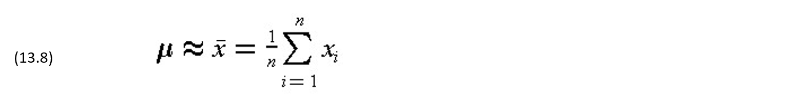
The fraction of defective items in a sample or the chance that the population average has different values is estimated from two statistics obtained from the sample: the sample mean and standard deviation. Mathematically, let n be the number of items in the sample and xi, i = 1,2,3,…,n, be the measured values of the variable characteristic x. Then an estimate of the overall population mean μ is the sample mean x :
An estimate of the population standard deviation is s, the square root of the sample variance statistic:
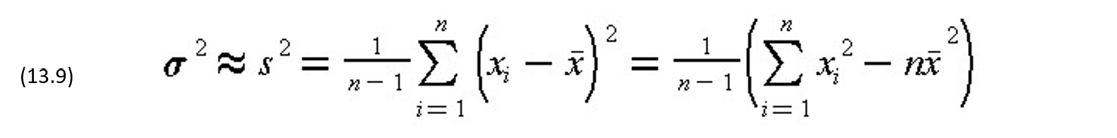
Based on these two estimated parameters and the desired limits, the various fractions of interest for the population can be calculated.
The probability that the average value of a population is greater than a particular lower limit is calculated from the test statistic:

which is t-distributed with n-1 degrees of freedom. If the population standard deviation is known in advance, then this known value is substituted for the estimate s and the resulting test statistic would be normally distributed. The t distribution is similar in appearance to a standard normal distribution, although the spread or variability in the function decreases as the degrees of freedom parameter increases. As the number of degrees of freedom becomes very large, the t-distribution coincides with the normal distribution.
With an upper limit, the calculations are similar, and the probability that the average value of a population is less than a particular upper limit can be calculated from the test statistic:

With both upper and lower limits, the sum of the probabilities of being above the upper limit or below the lower limit can be calculated.
The calculations to estimate the fraction of items above an upper limit or below a lower limit are very similar to those for the population average. The only difference is that the square root of the number of samples does not appear in the test statistic formulas:

and

where tAL is the test statistic for all items with a lower limit and tAU is the test statistic for all items with a upper limit. For example, the test statistic for items above an upper limit of 5.5 with x = 4.0, s = 3.0, and n = 5 is tAU = (8.5 – 4.0)/3.0 = 1.5 with n – 1 = 4 degrees of freedom.
Instead of using sampling plans that specify an allowable fraction of defective items, it saves computations to simply write specifications in terms of the allowable test statistic values themselves. This procedure is equivalent to requiring that the sample average be at least a pre-specified number of standard deviations away from an upper or lower limit. For example, with x = 4.0, U = 8.5, s = 3.0 and n = 41, the sample mean is only about (8.5 – 4.0)/3.0 = 1.5 standard deviations away from the upper limit.
To summarize, the application of sampling by variables requires the specification of a sample size, the relevant upper or limits, and either (1) the allowable fraction of items falling outside the designated limits or (2) the allowable probability that the population average falls outside the designated limit. Random samples are drawn from a pre-defined population and tested to obtained measured values of a variable attribute. From these measurements, the sample mean, standard deviation, and quality control test statistic are calculated. Finally, the test statistic is compared to the allowable trigger level and the lot is either accepted or rejected. It is also possible to apply sequential sampling in this procedure, so that a batch may be subjected to additional sampling and testing to further refine the test statistic values.
With sampling by variables, it is notable that a producer of material or work can adopt two general strategies for meeting the required specifications. First, a producer may ensure that the average quality level is quite high, even if the variability among items is high. This strategy is illustrated in Figure 13-3 as a “high quality average” strategy. Second, a producer may meet a desired quality target by reducing the variability within each batch. In Figure 13-3, this is labeled the “low variability” strategy. In either case, a producer should maintain high standards to avoid rejection of a batch.
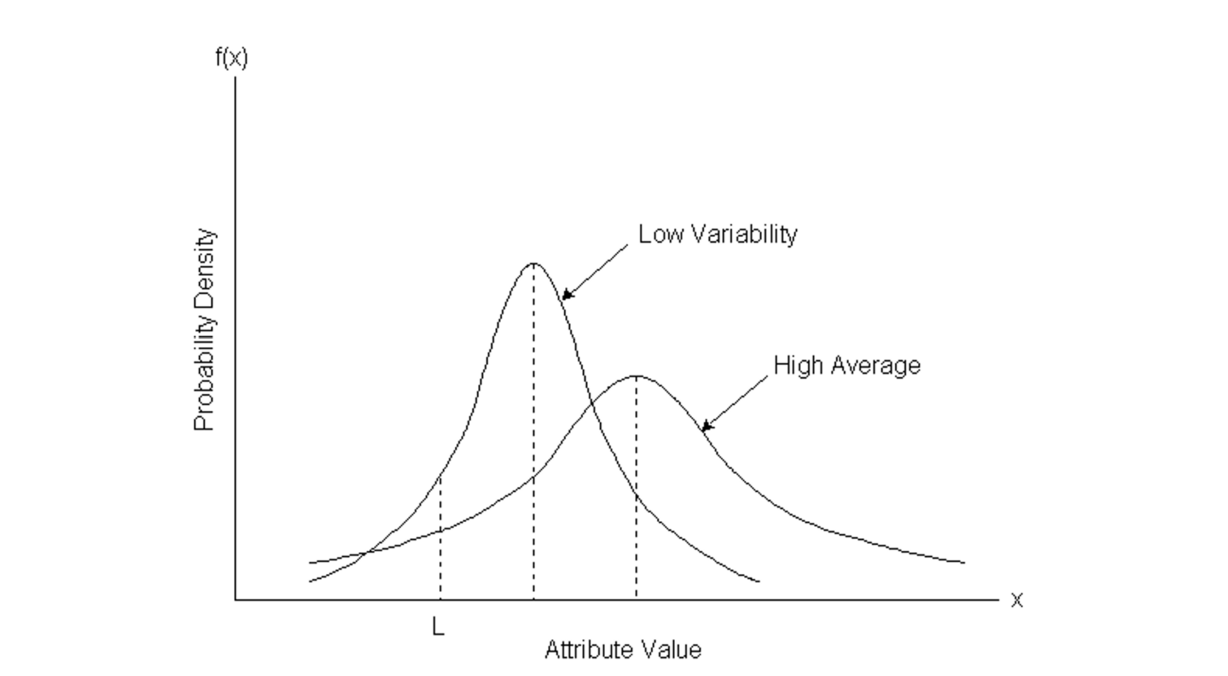
Figure 13-3 Testing for Defective Component Strengths
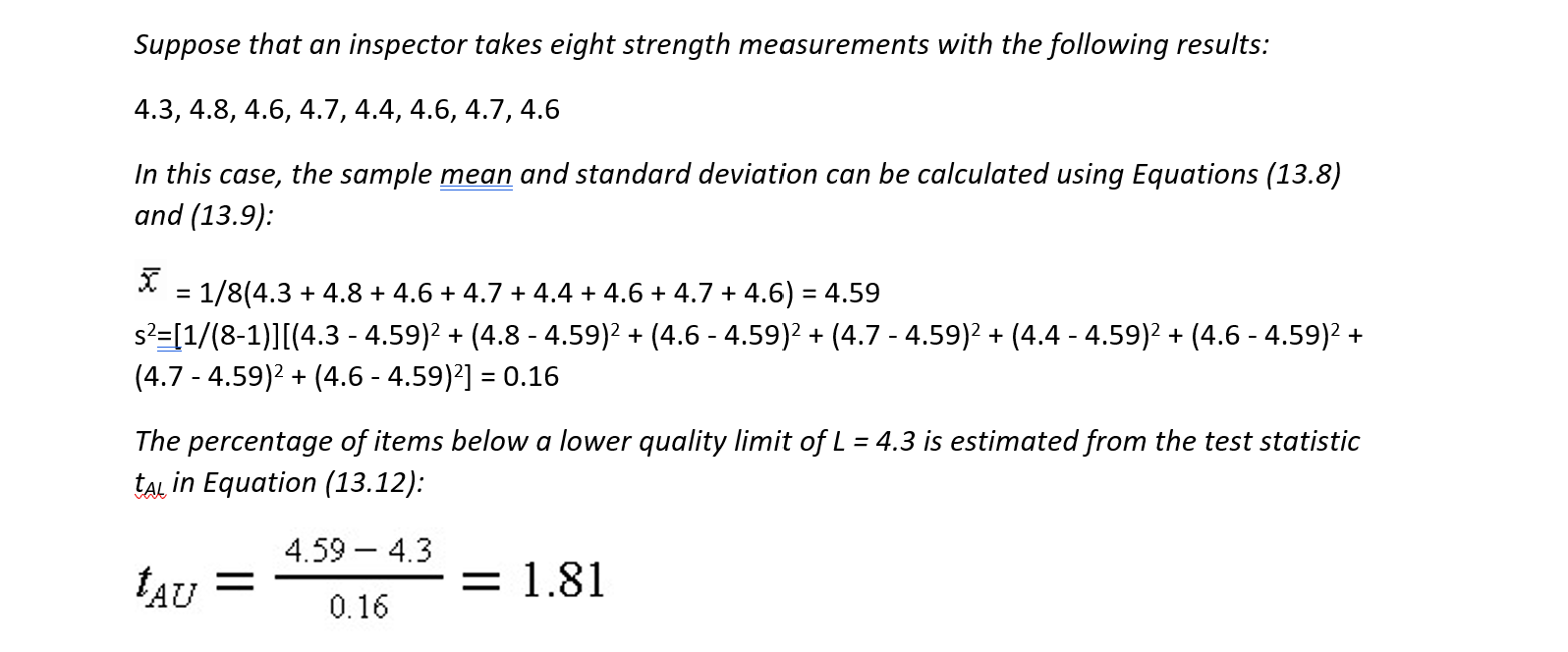
Example 13-5: Testing for defective component strengths
13.9 References
- Ang, A.H.S. and W.H. Tang, Probability Concepts in Engineering Planning and Design: Volume I – Basic Principles, John Wiley and Sons, Inc., New York, 1975.
- Au, T., R.M. Shane, and L.A. Hoel, Fundamentals of Systems Engineering: Probabilistic Models, Addison-Wesley Publishing Co., Reading MA, 1972
- Bowker, A.H. and Liebermann, G. J., Engineering Statistics, Prentice-Hall, 1972.
- Fox, A.J. and Cornell, H.A., (eds), Quality in the Constructed Project, American Society of Civil Engineers, New York, 1984.
- International Organization for Standardization, “Sampling Procedures and Charts for Inspection by Variables for Percent Defective, ISO 3951-1981 (E)”, Statistical Methods, ISO Standard Handbook 3, International Organization for Standardization, Paris, France, 1981.
- Skibniewski, M. and Hendrickson, C., Methods to Improve the Safety Performance of the U.S. Construction Industry, Technical Report, Department of Civil Engineering, Carnegie Mellon University, 1983.
- United States Department of Defense, Sampling Procedures and Tables for Inspection by Variables, (Military Standard 414), Washington D.C.: U.S. Government Printing Office, 1957.
- United States Department of Defense, Sampling Procedures and Tables for Inspection by Attributes, (Military Standard 105D), Washington D.C.: U.S. Government Printing Office, 1963.
13.10 Problems
(1) Consider the following specification. Would you consider it to be a process or performance specification? Why?
“Water used in mixing or curing shall be reasonably clean and free of oil, salt, acid, alkali, sugar, vegetable, or other substance injurious to the finished product…Water known to be potable quality may be used without test. Where the source of water is relatively shallow, the intake shall be so enclosed as to exclude silt, mud, grass, or other foreign materials.” [6]
(2) Suppose that a sampling plan calls for a sample of size n = 50. To be acceptable, only three or fewer samples can be defective. Estimate the probability of accepting the lot if the average defective percentage is (a) 15%, (b) 5% or (c) 2%. Do not use an approximation in this calculation.
(3) Repeat Problem 2 using the binomial approximation.
(4) Suppose that a project manager tested the strength of one tile out of a batch of 3,000 to be used on a building. This one sample measurement was compared with the design specification and, in this case, the sampled tile’s strength exceeded that of the specification. On this basis, the project manager accepted the tile shipment. If the sampled tile was defective (with a strength less than the specification), the project manager would have rejected the lot.
- What is the probability that ninety percent of the tiles are substandard, even though the project manager’s sample gave a satisfactory result?
- Sketch out the operating characteristic curve for this sampling plan as a function of the actual fraction of defective tiles.
(5) Repeat Problem 4 for sample sizes of (a) 5, (b) 10 and (c) 20.
(6) Suppose that a sampling-by-attributes plan is specified in which ten samples are taken at random from a large lot (N=100) and at most one sample item is allowed to be defective for the lot to be acceptable.
- If the actual percentage defective is five percent, what is the probability of lot acceptance? (Note: you may use relevant approximations in this calculation.)
- What is the consumer’s risk if an acceptable quality level is fifteen percent defective and the actual fraction defective is five percent?
- What is the producer’s risk with this sampling plan and an eight percent defective percentage?
(7) The yield stress of a random sample of 25 pieces of steel was measured, yielding a mean of 52,800 psi. and an estimated standard deviation of s = 4,600 psi.
- What is the probability that the population mean is less than 50,000 psi?
- What is the estimated fraction of pieces with yield strength less than 50,000 psi?
- Is this sampling procedure sampling-by-attributes or sampling-by-variable?
(8) Suppose that a contract specifies a sampling-by-attributes plan in which ten samples are taken at random from a large lot (N=100) and at most one sample is allowed to be defective for the lot to be acceptable.
- If the actual percentage defective is five percent, what is the probability of lot acceptance? (Note: you may use relevant approximations in this calculation).
- What is the consumer’s risk if an acceptable quality level is fifteen percent defective and the actual fraction defective is 0.05?
- What is the producer’s risk with this sampling plan and a 8% defective percentage?
(9) In a random sample of 40 blocks chosen from a production line, the mean length was 10.63 inches and the estimated standard deviation was 0.4 inch. Between what lengths can it be said that 98% of block lengths will lie?
13.11 Footnotes
- This illustrative pay factor schedule is adapted from R.M. Weed, “Development of Multicharacteristic Acceptance Procedures for Rigid Pavement,” Transportation Research Record 885, 1982, pp. 25-36. Back
- B.A. Gilly, A. Touran, and T. Asai, “Quality Control Circles in Construction,” ASCE Journal of Construction Engineering and Management, Vol. 113, No. 3, 1987, pg 432. Back
- See Improving Construction Safety Performance, Report A-3, The Business Roundtable, New York, NY, January 1982. Back
- Hinze, Jimmie W., Construction Safety,, Prentice-Hall, 1997. Back
- This example was adapted from E. Elinski, External Impacts of Reconstruction and Rehabilitation Projects with Implications for Project Management,Unpublished MS Thesis, Department of Civil Engineering, Carnegie Mellon University, 1985. Back
- American Association of State Highway and Transportation Officials, Guide Specifications for Highway Construction, Washington, D.C., Section 714.01, pg. 244. Back
