11 Advanced Scheduling Techniques
11.1 Use of Advanced Scheduling Techniques
The previous chapter described the fundamental scheduling techniques widely used and supported by numerous commercial scheduling systems. A variety of special techniques have also been developed to address specific circumstances or problems. While they come at the cost of more complexity and person-hours to implement, they are worthwhile in some cases. In this chapter, we survey some of the techniques that can be employed in this regard. These techniques address some important practical problems, such as:
- scheduling in the face of uncertain estimates on activity durations,
- integrated planning of scheduling and resource allocation,
- scheduling in unstructured or poorly formulated circumstances.
A final section in the chapter describes some possible improvements in the project scheduling process. In Chapter 14, we consider issues around integrating scheduling with other project management procedures.
11.2 Scheduling with Uncertain Durations
Section 10.3 described the application of critical path scheduling for the situation in which activity durations are fixed and known. Unfortunately, activity durations are estimates of the actual time required, and there is liable to be a significant amount of uncertainty associated with the actual durations. During the preliminary planning stages for a project, the uncertainty in activity durations is particularly large since the scope and obstacles to the project are still undefined. Activities that are outside of the control of the owner are likely to be more uncertain. For example, the time required to gain regulatory approval for projects may vary tremendously. Other external events such as adverse weather, trench collapses, or labor strikes make duration estimates particularly uncertain.
Two simple approaches to dealing with the uncertainty in activity durations warrant some discussion before introducing more formal scheduling procedures to deal with uncertainty. First, the uncertainty in activity durations may simply be ignored and scheduling done using the expected or most likely time duration for each activity. Since only one duration estimate needs to be made for each activity, this approach reduces the required work in setting up the original schedule. Formal methods of introducing uncertainty into the scheduling process require more work and assumptions. While this simple approach might be defended, it has two drawbacks. First, the use of expected activity durations typically results in overly optimistic schedules for completion; a numerical example of this optimism appears below. Second, the use of single activity durations often produces a rigid, inflexible mindset on the part of schedulers. As field managers appreciate, activity durations vary considerably and can be influenced by good leadership and close attention. As a result, field managers may lose confidence in the realism of a schedule based upon fixed activity durations. Clearly, the use of fixed activity durations in setting up a schedule makes a continual process of monitoring and updating the schedule in light of actual experience imperative. Otherwise, the project schedule is rapidly outdated.
A second simple approach to incorporating uncertainty also deserves mention. Many managers recognize that the use of expected durations may result in overly optimistic schedules, so they include a contingency allowance in their estimate of activity durations. For example, an activity with an expected duration of two days might be scheduled for a period of 2.2 days, including a ten percent contingency. Systematic application of this contingency would result in a ten percent increase in the expected time to complete the project. While the use of this rule-of-thumb or heuristic contingency factor can result in more accurate schedules, it is likely that formal scheduling methods that incorporate uncertainty more formally are useful as a means of obtaining greater accuracy or in understanding the effects of activity delays.
The most common formal approach to incorporate uncertainty in the scheduling process is to apply the critical path scheduling process (as described in Section 10.3) and then analyze the results from a probabilistic perspective. This process is usually referred to as the PERT scheduling or evaluation method. [1] PERT (Program Evaluation Review Technique) was introduced in 1957 to support the US Navy’s submarine building projects. Unfortunately, the term “PERT” has been used interchangeably with CPM scheduling over the years and in some user communities, however it is a distinct technique. As noted earlier, the duration of the critical path represents the minimum time required to complete the project. Using expected activity durations and critical path scheduling, a critical path of activities can be identified. This critical path is then used to analyze the duration of the project incorporating the uncertainty of the activity durations along the critical path. The expected project duration is equal to the sum of the expected durations of the activities along the critical path. Assuming that activity durations are independent random variables, the variance or variation in the duration of this critical path is calculated as the sum of the variances along the critical path. With the mean and variance of the identified critical path known, the distribution of activity durations can also be computed.
The mean and variance for each activity duration are typically computed from estimates of “optimistic” (ai,j), “most likely” (mi,j), and “pessimistic” (bi,j) activity durations using the formulas:
(11.1) μ(i,j) = 1/6( ai,j + 4mi,j + bi,j )
and
(11.2) σ2(i,j) = 1/36( bi,j – ai,j )2
where μ(i,j) and σ2(i,j) are the mean duration and its variance, respectively, of an activity (i,j). Three activity durations estimates (i.e., optimistic, most likely, and pessimistic durations) are required in the calculation. The use of these optimistic, most likely, and pessimistic estimates stems from the fact that these are thought to be easier for managers to estimate subjectively. The formulas for calculating the mean and variance are derived by assuming that the activity durations follow a probabilistic beta distribution under a restrictive condition. [2] The probability density function of a beta distributions for a random variable x is given by:
(11.3) f(x) = k( x – a )α ( b – x)β
a ≤ x ≤ b and α, β > -1
where k is a constant which can be expressed in terms of α and β. Several beta distributions for different sets of values of α and β are shown in Figure 11-1. For a beta distribution in the interval a ≤ x ≤ b having a modal value m, the mean is given by:
(11.4) μ = ( a + (α + β)m + b ) / ( α + β + 2)
If α + β = 4, then Eq. (11.4) will result in Eq. (11.1). Thus, the use of Eqs. (11.1) and (11.2) impose an additional condition on the beta distribution. In particular, the restriction that σ = (b – a)/6 is imposed.
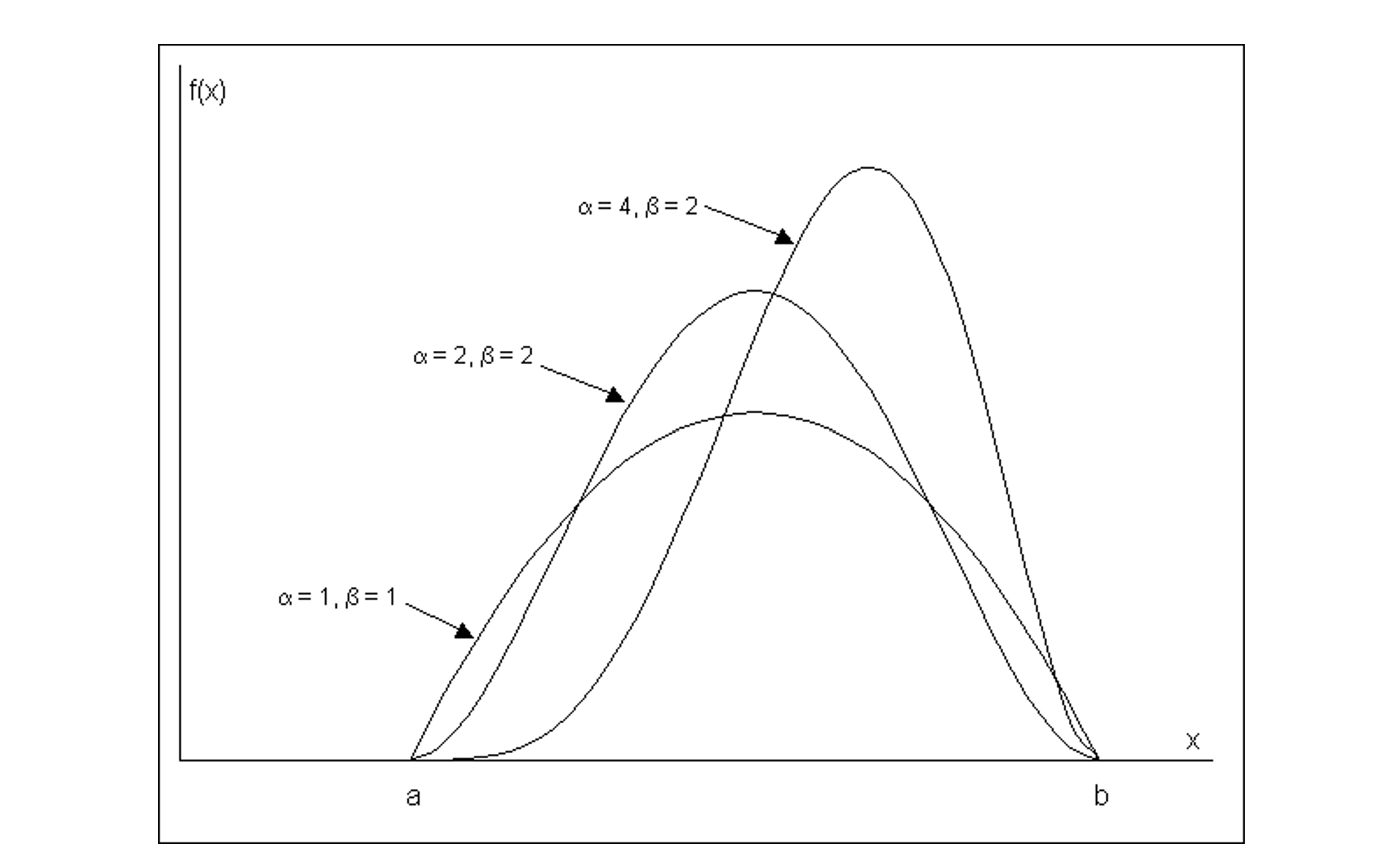
Figure 11-1 Illustration of Several Beta Distributions
Since absolute limits on the optimistic and pessimistic activity durations are extremely difficult to estimate from historical data, a common practice is to use the ninety-fifth percentile of activity durations for these points. Thus, the optimistic time would be such that there is only a one in twenty (five percent) chance that the actual duration would be less than the estimated optimistic time. Similarly, the pessimistic time is chosen so that there is only a five percent chance of exceeding this duration. Thus, there is a ninety percent chance of having the actual duration of an activity fall between the optimistic and pessimistic duration time estimates. With the use of ninety-fifth percentile values for the optimistic and pessimistic activity durations, the calculation of the expected duration according to Eq. (11.1) is unchanged but the formula for calculating the activity variance becomes:

The difference between Eqs. (11.2) and (11.5) comes only in the value of the divisor, with 36 used for absolute limits and 10 used for ninety-five percentile limits. This difference might be expected since the difference between bi,j and ai,j would be larger for absolute limits than for the ninety-fifth percentile limits.
While the PERT method has been made widely available, it suffers from three major problems. First, the procedure focuses upon a single critical path, when many paths might become critical due to random fluctuations. For example, suppose that the critical path with longest expected time happened to be completed early. Unfortunately, this does not necessarily mean that the project is completed early since another path or sequence of activities might take longer. Similarly, a longer than expected duration for an activity not on the critical path might result in that activity suddenly becoming critical. As a result of the focus on only a single path, the PERT method typically underestimates the actual project duration.
As a second problem with the PERT procedure, it is incorrect to assume that most construction activity durations are independent random variables. In practice, durations are correlated with one another. For example, if problems are encountered in the delivery of concrete for a project, this problem is likely to influence the expected duration of numerous activities involving concrete pours on a project. Positive correlations of this type between activity durations imply that the PERT method underestimates the variance of the critical path and thereby produces over-optimistic expectations of the probability of meeting a particular project completion deadline.
Finally, the PERT method requires three duration estimates for each activity rather than the single estimate developed for critical path scheduling. Thus, the difficulty and labor of estimating activity characteristics is multiplied threefold.
As an alternative to the PERT procedure, a straightforward method of obtaining information about the distribution of project completion times (as well as other schedule information) is through the use of Monte Carlo simulation. This technique calculates sets of artificial (but realistic) activity duration times and then applies a deterministic scheduling procedure to each set of durations. Numerous calculations are required in this process since simulated activity durations must be calculated and the scheduling procedure applied many times. For realistic project networks, 40 to 1,000 separate sets of activity durations might be used in a single scheduling simulation run. The calculations associated with Monte Carlo simulation are described in the following section. Many software packages exist to run Monte Carlo simulations. One that the author has used and which is still widely used at the last date of revision of this text is Lumivero’s @RISK and Decision Tools SuiteTM software which integrates smoothly with MS ProjectTM and PrimaveraTM.
A number of different indicators of the project schedule can be estimated from the results of a Monte Carlo simulation:
- Estimates of the expected time and variance of the project completion.
- An estimate of the distribution of completion times, so that the probability of meeting a particular completion date can be estimated.
- The probability that a particular activity will lie on the critical path. This is of interest since the longest or critical path through the network may change as activity durations change.
The disadvantage of Monte Carlo simulation results from the additional information about activity durations that is required and the computational effort involved in numerous scheduling applications for each set of simulated durations. For each activity, the distribution of possible durations as well as the parameters of this distribution must be specified. For example, durations might be assumed or estimated to be uniformly distributed between a lower and upper value. In addition, correlations between activity durations should be specified. For example, if two activities involve assembling forms in different locations and at different times for a project, then the time required for each activity is likely to be closely related. If the forms pose some problems, then assembling them on both occasions might take longer than expected. This is an example of a positive correlation in activity times. In application, such correlations are commonly ignored, leading to errors in results. As a final problem and discouragement, easy to use software systems for Monte Carlo simulation of project schedules are not generally available. This is particularly the case when correlations between activity durations are desired. An analysis by Shahtaheri, published in 2016, of the planned retubing and refurbishment work of the type being completed at the Darlington, Pickering and Bruce nuclear power stations in Ontario (at the costs of tens of billions of Canadian dollars in the 2020-2030 time frame) did combine such interdependencies (identified as common risks) and activity duration uncertainties into a comprehensive JCL (joint confidence limit ) analysis for project duration, cost and radiation exposure. It was used to inform a class five estimate of the planned work.
Another approach to the simulation of different activity durations is to develop specific scenarios of events and determine the effect on the overall project schedule. This is a type of “what-if” problem solving in which a manager simulates events that might occur and sees the result. For example, the effects of different weather patterns on activity durations could be estimated and the resulting schedules for the different weather patterns compared. One method of obtaining information about the range of possible schedules is to apply the scheduling procedure using all optimistic, all most likely, and then all pessimistic activity durations. The result is three project schedules representing a range of possible outcomes. This process of “what-if” analysis is similar to that undertaken during the process of construction planning or during analysis of project crashing.
Example 11-1: Scheduling activities with uncertain time durations.
Suppose that the nine-activity example project shown in Table 10-2 and Figure 10-4 of Chapter 10 was thought to have very uncertain activity time durations. As a result, project scheduling considering this uncertainty is desired. All three methods (PERT, Monte Carlo simulation, and “What-if” simulation) will be applied.
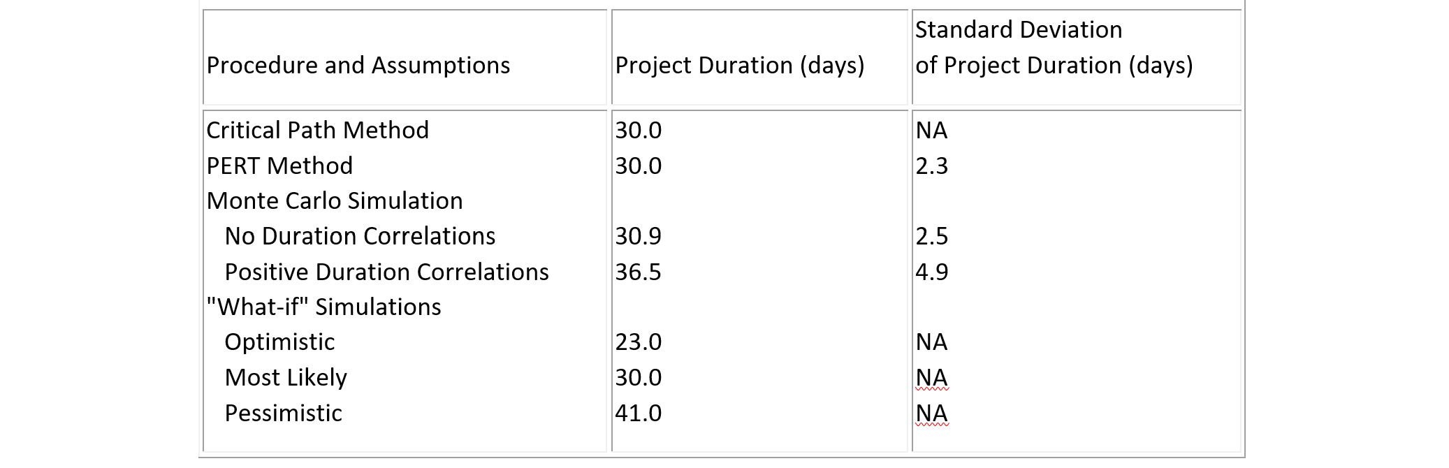
Table 11-1 shows the estimated optimistic, most likely and pessimistic durations for the nine activities. From these estimates, the mean, variance and standard deviation are calculated. In this calculation, ninety-fifth percentile estimates of optimistic and pessimistic duration times are assumed, so that Equation (11.5) is applied. The critical path for this project ignoring uncertainty in activity durations consists of activities A, C, F and I as found in Table 10-3 (Section 10.3). Applying the PERT analysis procedure suggests that the duration of the project would be approximately normally distributed. The sum of the means for the critical activities is 4.0 + 8.0 + 12.0 + 6.0 = 30.0 days, and the sum of the variances is 0.4 + 1.6 + 1.6 + 1.6 = 5.2 leading to a standard deviation of 2.3 days.
With a normally distributed project duration, the probability of meeting a project deadline is equal to the probability that the standard normal distribution is less than or equal to (PD – μD)|σD where PD is the project deadline, μD is the expected duration and σD is the standard deviation of project duration. For example, the probability of project completion within 35 days is:
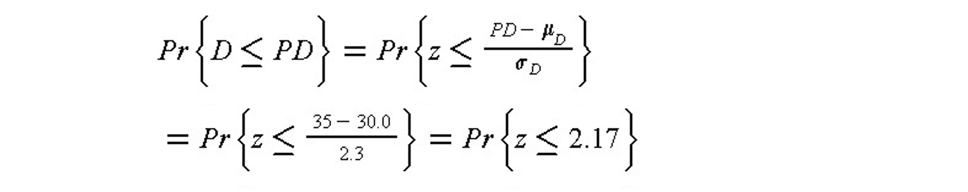
where z is the standard normal distribution tabulated value of the cumulative standard distribution appears in Table B.1 of Appendix B.
Monte Carlo simulation results provide slightly different estimates of the project duration characteristics. Assuming that activity durations are independent and approximately normally distributed random variables with the mean and variances shown in Table 11-1, a simulation can be performed by obtaining simulated duration realization for each of the nine activities and applying critical path scheduling to the resulting network. Applying this procedure 500 times, the average project duration is found to be 30.9 days with a standard deviation of 2.5 days. The PERT result is less than this estimate by 0.9 days or three percent. Also, the critical path considered in the PERT procedure (consisting of activities A, C, F and I) is found to be the critical path in the simulated networks less than half the time.
TABLE 11-1 Activity Duration Estimates for a Nine Activity Project
| Activity | Optimistic Duration | Most Likely Duration | Pessimistic Duration | Mean | Variance |
| A B C D E F G H I |
3 2 6 5 6 10 2 4 4 |
4 3 8 7 9 12 2 5 6 |
5 5 10 8 14 14 4 8 8 |
4.0 3.2 8.0 6.8 9.3 12.0 2.3 5.3 6.0 |
0.4 0.9 1.6 0.9 6.4 1.6 0.4 1.6 1.6 |
If there are correlations among the activity durations, then significantly different results can be obtained. For example, suppose that activities C, E, G and H are all positively correlated random variables with a correlation of 0.5 for each pair of variables. Applying Monte Carlo simulation using 500 activity network simulations results in an average project duration of 36.5 days and a standard deviation of 4.9 days. This estimated average duration is 6.5 days or 20 percent longer than the PERT estimate or the estimate obtained ignoring uncertainty in durations. If correlations like this exist, these methods can seriously underestimate the actual project duration.
Finally, the project durations obtained by assuming all optimistic and all pessimistic activity durations are 23 and 41 days respectively. Other “what-if” simulations might be conducted for cases in which peculiar soil characteristics might make excavation difficult; these soil peculiarities might be responsible for the correlations of excavation activity durations described above.
Results from the different methods are summarized in Table 11-2. Note that positive correlations among some activity durations results in relatively large increases in the expected project duration and variability.
TABLE 11-2 Project Duration Results from Various Techniques and Assumptions for an Example
11.3 Calculations for Monte Carlo Schedule Simulation
In this section, we outline the procedures required to perform Monte Carlo simulation for the purpose of schedule analysis. These procedures presume that the various steps involved in forming a network plan and estimating the characteristics of the probability distributions for the various activities have been completed. Given a plan and the activity duration distributions, the heart of the Monte Carlo simulation procedure is the derivation of a realization or synthetic outcome of the relevant activity durations. Once these realizations are generated, standard scheduling techniques can be applied. We shall present the formulas associated with the generation of normally distributed activity durations, and then comment on the requirements for other distributions in an example.
To generate normally distributed realizations of activity durations, we can use a two-step procedure. First, we generate uniformly distributed random variables, ui in the interval from zero to one. Numerous techniques can be used for this purpose. For example, a general formula for random number generation can be of the form:

where π = 3.14159265 and ui-1 was the previously generated random number or a pre-selected beginning or seed number. For example, a seed of u0 = 0.215 in Eq. (11.6) results in u1 = 0.0820, and by applying this value of u1, the result is u2 = 0.1029. This formula is a special case of the mixed congruential method of random number generation. While Equation (11.6) will result in a series of numbers that have the appearance and the necessary statistical properties of true random numbers, we should note that these are actually “pseudo” random numbers since the sequence of numbers will repeat given a long enough time.
With a method of generating uniformly distributed random numbers, we can generate normally distributed random numbers using two uniformly distributed realizations with the equations: [3]
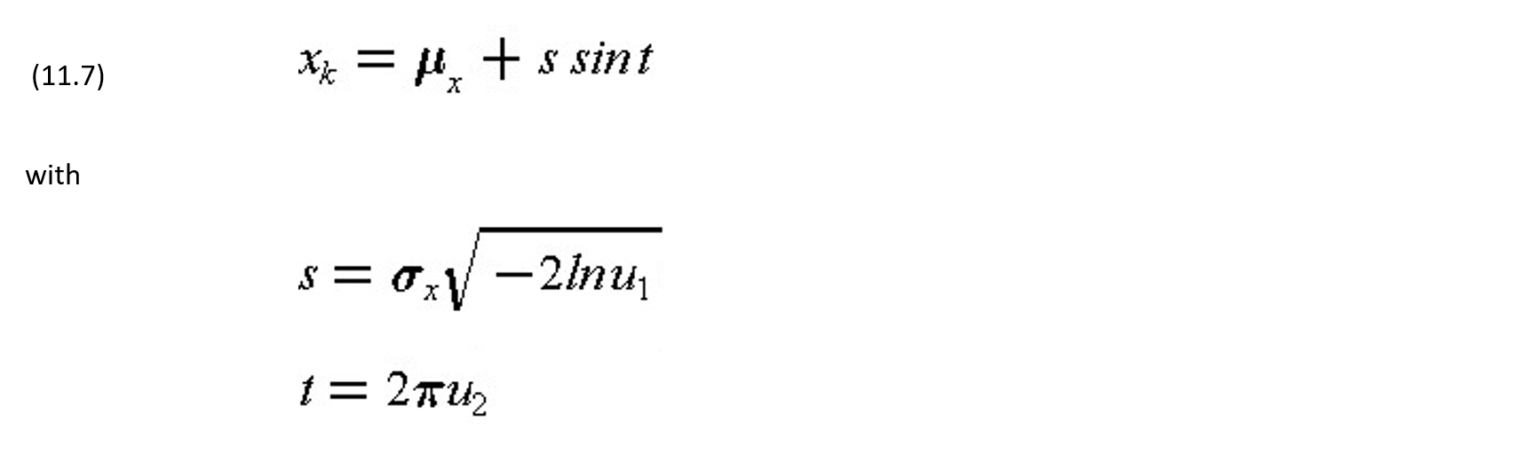
where xk is the normal realization, μx is the mean of x, σx is the standard deviation of x, and u1 and u2 are the two uniformly distributed random variable realizations. For the case in which the mean of an activity is 2.5 days and the standard deviation of the duration is 1.5 days, a corresponding realization of the duration is s = 2.2365, t = 0.6465 and xk = 2.525 days, using the two uniform random numbers generated from a seed of 0.215 above.
Correlated random number realizations may be generated making use of conditional distributions. For example, suppose that the duration of an activity d is normally distributed and correlated with a second normally distributed random variable x which may be another activity duration or a separate factor such as a weather effect. Given a realization xk of x, the conditional distribution of d is still normal, but it is a function of the value xk. In particular, the conditional mean (μ‘d | x = xk) and standard deviation (σ‘d | x = xk) of a normally distributed variable given a realization of the second variable is:

where ρdx is the correlation coefficient between d and x. Once xk is known, the conditional mean and standard deviation can be calculated from Eq. (11.8) and then a realization of d obtained by applying Equation (11.7).
Correlation coefficients indicate the extent to which two random variables will tend to vary together. Positive correlation coefficients indicate one random variable will tend to exceed its mean when the other random variable does the same. From a set of n historical observations of two random variables, x and y, the correlation coefficient can be estimated as:

The value of ρxy can range from one to minus one, with values near one indicating a positive, near linear relationship between the two random variables.
It is also possible to develop formulas for the conditional distribution of a random variable correlated with numerous other variables; this is termed a multi-variate distribution. [4] Random number generations from other types of distributions are also possible. [5] Once a set of random variable distributions is obtained, then the process of applying a scheduling algorithm is required as described in previous sections.
Example 11-2: A Three-Activity Project Example
Suppose that we wish to apply a Monte Carlo simulation procedure to a simple project involving three activities in series. As a result, the critical path for the project includes all three activities. We assume that the durations of the activities are normally distributed with the following parameters:
| Activity | Mean (Days) | Standard Deviation (Days) |
| A B C |
2.5 5.6 2.4 |
1.5 2.4 2.0 |
To simulate the schedule effects, we generate the duration realizations shown in Table 11-3 and calculate the project duration for each set of three activity duration realizations.
For the twelve sets of realizations shown in the table, the mean and standard deviation of the project duration can be estimated to be 10.49 days and 4.06 days respectively. In this simple case, we can also obtain an analytic solution for this duration, since it is only the sum of three independent normally distributed variables. The actual project duration has a mean of 10.5 days, and a standard deviation of ( (1.5)2 + (2.4)2 + (2.0)2 ).5 = 3.5 days. With only a limited number of simulations, the mean obtained from simulations is close to the actual mean, while the estimated standard deviation from the simulation differs significantly from the actual value. This latter difference can be attributed to the nature of the set of realizations used in the simulations; using a larger number of simulated durations would result in a more accurate estimate of the standard deviation.
TABLE 11-3 Duration Realizations for a Monte Carlo Schedule Simulation
| Simulation Number | Activity A | Activity B | Activity C | Project Duration |
| 1 2 3 4 5 6 7 8 9 10 11 12 |
1.53 2.67 3.36 0.39 2.50 2.77 3.83 3.73 1.06 1.17 1.68 0.37 |
6.94 4.83 6.86 7.65 5.82 8.71 2.05 10.57 3.68 0.86 9.47 6.66 |
1.04 2.17 5.56 2.17 1.74 4.03 1.10 3.24 2.47 1.37 0.13 1.70 |
9.51 9.66 15.78 10.22 10.06 15.51 6.96 17.53 7.22 3.40 11.27 8.72 |
| Estimated Mean Project Duration = 10.49 Estimated Standard Deviation of Project Duration = 4.06 |
Note: All durations in days.
Example 11-3: Generation of Realizations from Triangular Distributions
To simplify calculations for Monte Carlo simulation of schedules, the use of a triangular distribution is advantageous compared to the normal or the beta distributions. Triangular distributions also have the advantage relative to the normal distribution that negative durations cannot be estimated. As illustrated in Figure 11-2, the triangular distribution can be skewed to the right or left and has finite limits like the beta distribution. If a is the lower limit, b the upper limit and m the most likely value, then the mean and standard deviation of a triangular distribution are:

The cumulative probability function for the triangular distribution is:
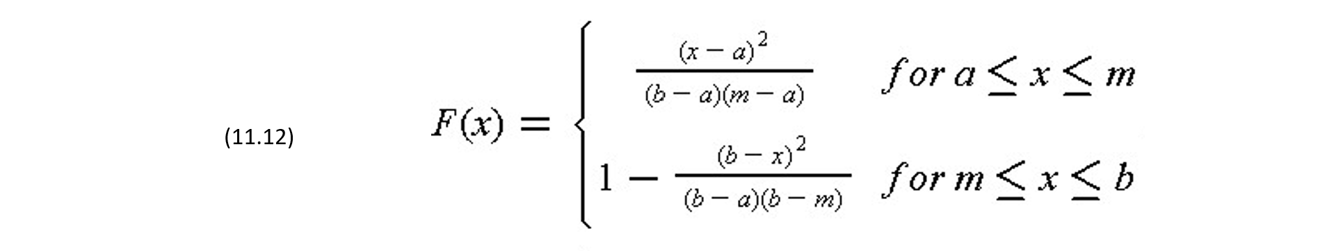
where F(x) is the probability that the random variable is less than or equal to the value of x.
Figure 11-2 Illustration of Two Triangular Activity Duration Distributions
Generating a random variable from this distribution can be accomplished with a single uniform random variable realization using the inversion method. In this method, a realization of the cumulative probability function, F(x) is generated and the corresponding value of x is calculated. Since the cumulative probability function varies from zero to one, the density function realization can be obtained from the uniform value random number generator, Equation (11.6). The calculation of the corresponding value of x is obtained from inverting Equation (11.12):

For example, if a = 3.2, m = 4.5 and b = 6.0, then μx = 4.8 and σx = 2.7. With a uniform realization of u = 0.215, then for (m-a)/(b-a) ≥ 0.215, x will lie between a and m and is found to have a value of 4.1 from Equation (11.13).
11.4 Crashing and Time/Cost Trade-offs
The previous sections discussed the duration of activities as either fixed or random numbers with known characteristics. However, activity durations can often vary depending upon the type and amount of resources that are applied. Assigning more workers to a particular activity will normally result in a shorter duration. [6] Greater speed may result in higher costs and lower quality, however. In this section, we shall consider the impacts of time, cost and quality trade-offs in activity durations. In this process, we shall discuss the procedure of project crashing as described below.
A simple representation of the possible relationship between the duration of an activity and its direct costs appears in Figure 11-3. Considering only this activity in isolation and without reference to the project completion deadline, a manager would undoubtedly choose a duration which implies minimum direct cost, represented by Dij and Cij in the figure. Unfortunately, if each activity was scheduled for the duration that resulted in the minimum direct cost in this way, the time to complete the entire project might be too long and substantial penalties associated with the late project start-up might be incurred. This is a small example of sub-optimization, in which a small component of a project is optimized or improved to the detriment of the entire project performance. Avoiding this problem of sub-optimization is a fundamental concern of project managers.
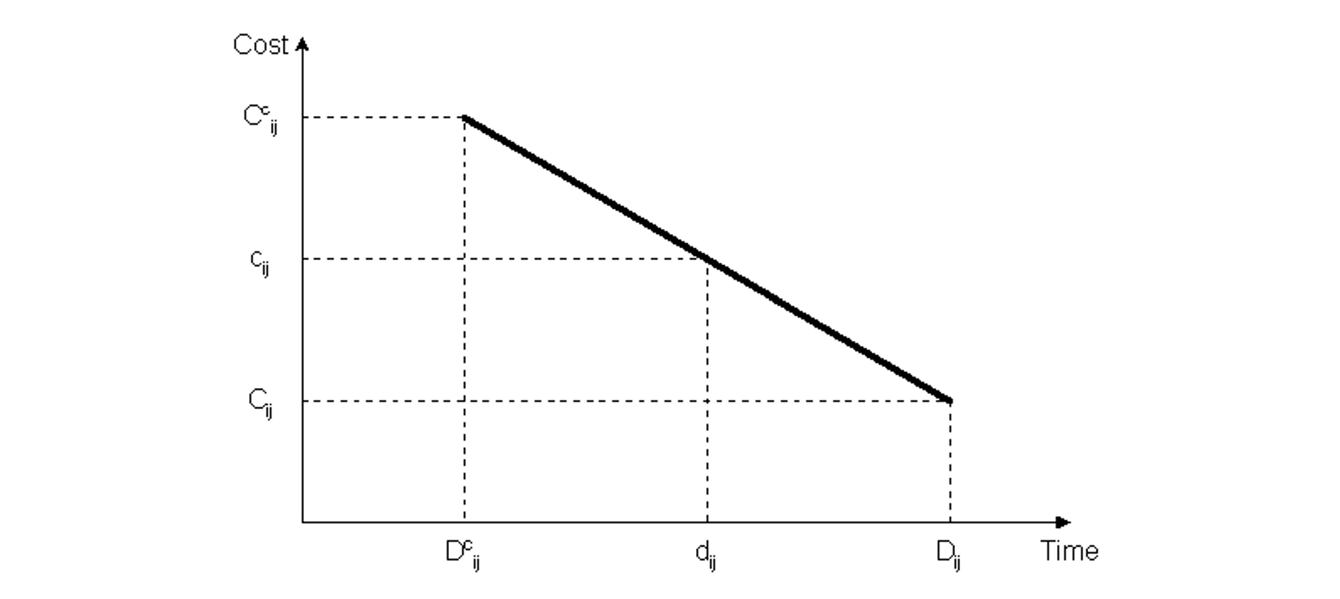
Figure 11-3 Illustration of a Linear Time/Cost Trade-off for an Activity
At the other extreme, a manager might choose to complete the activity in the minimum possible time, Dcij, but at a higher cost Ccij. This minimum completion time is commonly called the activity crash time. The linear relationship shown in the figure between these two points implies that any intermediate duration could also be chosen. It is possible that some intermediate point may represent the ideal or optimal trade-off between time and cost for this activity.
What is the reason for an increase in direct cost as the activity duration is reduced? A simple case arises in the use of overtime work. By scheduling weekend or evening work, the completion time for an activity as measured in calendar days will be reduced. However, premium wages must be paid for such overtime work, so the cost will increase. Also, overtime work is more prone to accidents and quality problems that must be corrected, so indirect costs may also increase. More generally, we might not expect a linear relationship between duration and direct cost, but some convex function such as the nonlinear curve or the step function shown in Figure 11-4. A linear function may be a good approximation to the actual curve, however, and results in considerable analytical simplicity. [7]
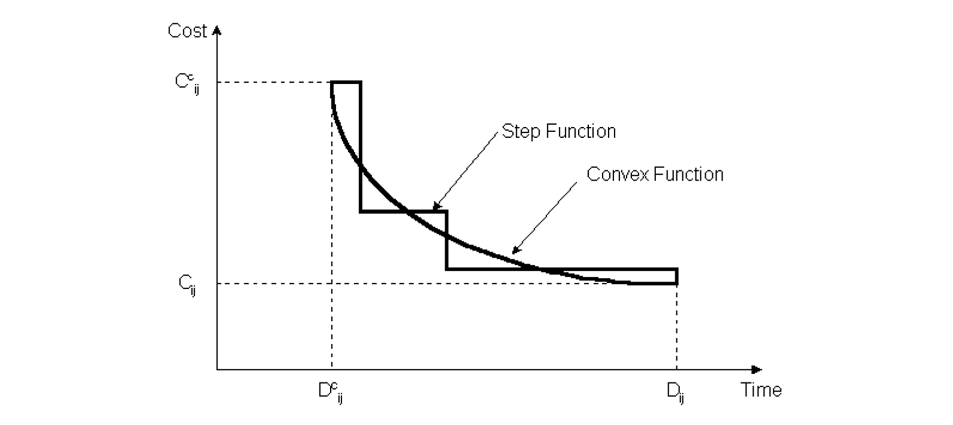
Figure 11-4 Illustration of Non-linear Time/Cost Trade-offs for an Activity
With a linear relationship between cost and duration, the critical path time/cost trade-off problem can be defined as a linear programming optimization problem. In particular, let Rij represent the rate of change of cost as duration is decreased, illustrated by the absolute value of the slope of the line in Figure 11-3. Then, the direct cost of completing an activity is:

where the lower case cij and dij represent the scheduled duration and resulting cost of the activity ij. The actual duration of an activity must fall between the minimum cost time (Dij) and the crash time (Dcij). Also, precedence constraints must be imposed as described earlier for each activity. Finally, the required completion time for the project or, alternatively, the costs associated with different completion times must be defined. Thus, the entire scheduling problem is to minimize total cost (equal to the sum of the cij values for all activities) subject to constraints arising from (1) the desired project duration, PD, (2) the minimum and maximum activity duration possibilities, and (3) constraints associated with the precedence or completion times of activities. Algebraically, this is:
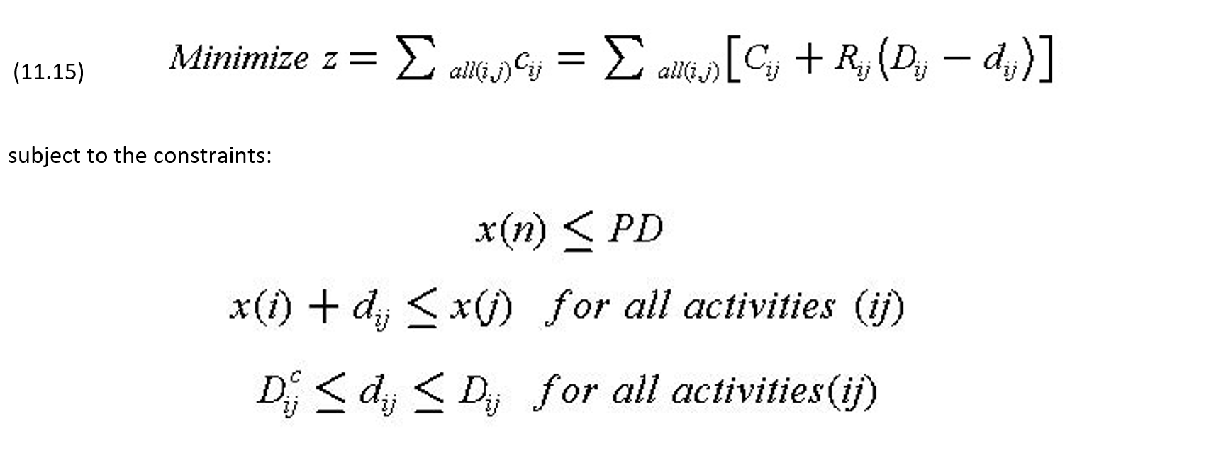
where the notation is defined above, and the decision variables are the activity durations dij and event times x(k). The appropriate schedules for different project durations can be found by repeatedly solving this problem for different project durations PD. The entire problem can be solved by linear programming or more efficient algorithms which take advantage of the special network form of the problem constraints. Genetic algorithms, AI techniques, and constraint-based optimization have also been applied to solving problems of this sort.
One solution to the time-cost trade-off problem is of particular interest and deserves mention here. The minimum time to complete a project is called the project-crash time. This minimum completion time can be found by applying critical path scheduling with all activity durations set to their minimum values (Dcij). This minimum completion time for the project can then be used in the time-cost scheduling problem described above to determine the minimum project-crash cost. Note that the project crash cost is not found by setting each activity to its crash duration and summing up the resulting costs; this solution is called the all-crash cost. Since there are some activities not on the critical path that can be assigned longer duration without delaying the project, it is advantageous to change the all-crash schedule and thereby reduce costs.
Heuristic approaches are also possible to the time/cost trade-off problem. In particular, a simple approach is to first apply critical path scheduling with all activity durations assumed to be at minimum cost (Dij). Next, the planner can examine activities on the critical path and reduce the scheduled duration of activities which have the lowest resulting increase in costs. In essence, the planner develops a list of activities on the critical path ranked in accordance with the unit change in cost for a reduction in the activity duration. The heuristic solution proceeds by shortening activities in the order of their lowest impact on costs. As the duration of activities on the shortest path are shortened, the project duration is also reduced. Eventually, another path becomes critical, and a new list of activities on the critical path must be prepared. By manual or automatic adjustments of this kind, good but not necessarily optimal schedules can be identified. Optimal or best schedules can only be assured by examining changes in combinations of activities as well as changes to single activities. However, by alternating between adjustments in particular activity durations (and their costs) and a critical path scheduling procedure, a planner can fairly rapidly devise a shorter schedule to meet a particular project deadline or, in the worst case, find that the deadline is impossible of accomplishment.
This type of heuristic approach to time-cost trade-offs is essential when the time-cost trade-offs for each activity are not known in advance or in the case of resource constraints on the project. In these cases, heuristic explorations may be useful to determine if greater effort should be spent on estimating time-cost trade-offs or if additional resources should be retained for the project. In many cases, the basic time/cost trade-off might not be a smooth curve as shown in Figure 11-4, but only a series of particular resource and schedule combinations which produce particular durations. For example, a planner might have the option of assigning either one or two crews to a particular activity; in this case, there are only two possible durations of interest.
Example 11-4: Time/Cost Trade-offs
The construction of a permanent transitway on an expressway median illustrates the possibilities for time/cost trade-offs in construction work. [8] One section of 10 miles of transitway was built in 1985 and 1986 to replace an existing contra-flow lane system (in which one lane in the expressway was reversed each day to provide additional capacity in the peak flow direction). Three engineers’ estimates for work time were prepared:
-
- 975 calendar day, based on 750 working days at 5 days/week and 8 hours/day of work plus 30 days for bad weather, weekends and holidays.
- 702 calendar days, based on 540 working days at 6 days/week and 10 hours/day of work.
- 360 calendar days, based on 7 days/week and 24 hours/day of work.
The savings from early completion due to operating savings in the contra-flow lane and contract administration costs were estimated to be $5,000 per day.
In accepting bids for this construction work, the owner required both a dollar amount and a completion date. The bidder’s completion date was required to fall between 360 and 540 days. In evaluating contract bids, a $5,000 credit was allowed for each day less than 540 days that a bidder specified for completion. In the end, the successful bidder completed the project in 270 days, receiving a bonus of 5,000*(540-270) = $450,000 in the $8,200,000 contract. However, the contractor experienced fifteen to thirty percent higher costs to maintain the continuous work schedule.
Example 11-5: Time cost trade-offs and project crashing
As an example of time/cost trade-offs and project crashing, suppose that we needed to reduce the project completion time for a seven-activity product delivery project first analyzed in Section 10.3 as shown in Table 10-4 and Figure 10-7. Table 11-4 gives information pertaining to possible reductions in time which might be accomplished for the various activities. Using the minimum cost durations (as shown in column 2 of Table 11-4), the critical path includes activities C,E,F,G plus a dummy activity X. The project duration is 32 days in this case, and the project cost is $70,000.
TABLE 11-4 Activity Durations and Costs for a Seven Activity Project
| Activity | Minimum Cost | Normal Duration | Crash Cost | Crash Duration | Change in Cost per Day |
| A B C D E F G |
8 4 8 10 10 20 10 |
6 1 8 5 9 12 3 |
14 4 24 24 18 36 18 |
4 1 4 3 5 6 2 |
3 — 4 7 2 2.7 8 |
Examining the unit change in cost, Rij shown in column 6 of Table 11-4, the lowest rate of change occurs for activity E. Accordingly, a good heuristic strategy might be to begin by crashing this activity. The result is that the duration of activity E goes from 9 days to 5 days and the total project cost increases by $8,000. After making this change, the project duration drops to 28 days and two critical paths exist: (1) activities C,X,E,F and G, and (2) activities C, D, F, and G.
Examining the unit changes in cost again, activity F has the lowest value of Rijj. Crashing this activity results in an additional time savings of 6 days in the project duration, an increase in project cost of $16,000, but no change in the critical paths. The activity on the critical path with the next lowest unit change in cost is activity C. Crashing this activity to its minimum completion time would reduce its duration by 4 days at a cost increase of $16,000. However, this reduction does not result in a reduction in the duration of the project by 4 days. After activity C is reduced to 7 days, then the alternate sequence of activities A and B lie on the critical path and further reductions in the duration of activity C alone do not result in project time savings. Accordingly, our heuristic corrections might be limited to reducing activity C by only 1 day, thereby increasing costs by $4,000 and reducing the project duration by 1 day.
At this point, our choices for reducing the project duration are fairly limited. We can either reduce the duration of activity G or, alternatively, reduce activity C and either activity A or activity B by an identical amount. Inspection of Table 11-4 and Figure 10-4 suggest that reducing activity A and activity C is the best alternative. Accordingly, we can shorten activity A to its crash duration (from 6 days to 4 days) and shorten the duration of activity C (from 7 days to 5 days) at an additional cost of $6,000 + $8,000 = $14,000. The result is a reduction in the project duration of 2 days.
Our last option for reducing the project duration is to crash activity G from 3 days to 2 days at an increase in cost of $8,000. No further reductions are possible in this time since each activity along a critical path (comprised of activities A, B, E, F and G) are at minimum durations. At this point, the project duration is 18 days and the project cost is $120,000., representing a fifty percent reduction in project duration and a seventy percent increase in cost. Note that not all the activities have been crashed. Activity C has been reduced in duration to 5 days (rather than its 4 day crash duration), while activity D has not been changed at all. If all activities had been crashed, the total project cost would have been $138,000, representing a useless expenditure of $18,000. The change in project cost with different project durations is shown graphically in Figure 11-5.
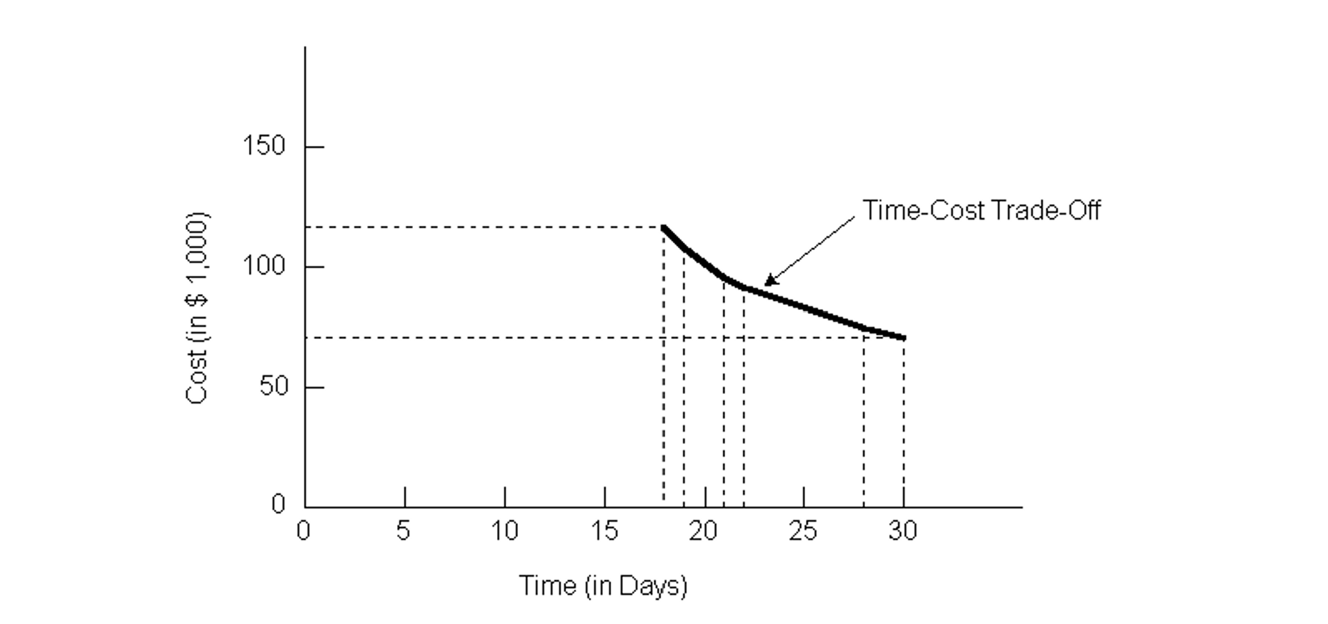
Figure 11-5 Project Cost Versus Time for a Seven Activity Project
Example 11-8: Mathematical Formulation of Time-Cost Trade-offs
The same results obtained in the previous example could be obtained using a formal optimization program and the data appearing in Tables 10-4 and 11-4. In this case, the heuristic approach used above has obtained the optimal solution at each stage. Using Eq. (11.15), the linear programming problem formulation would be:
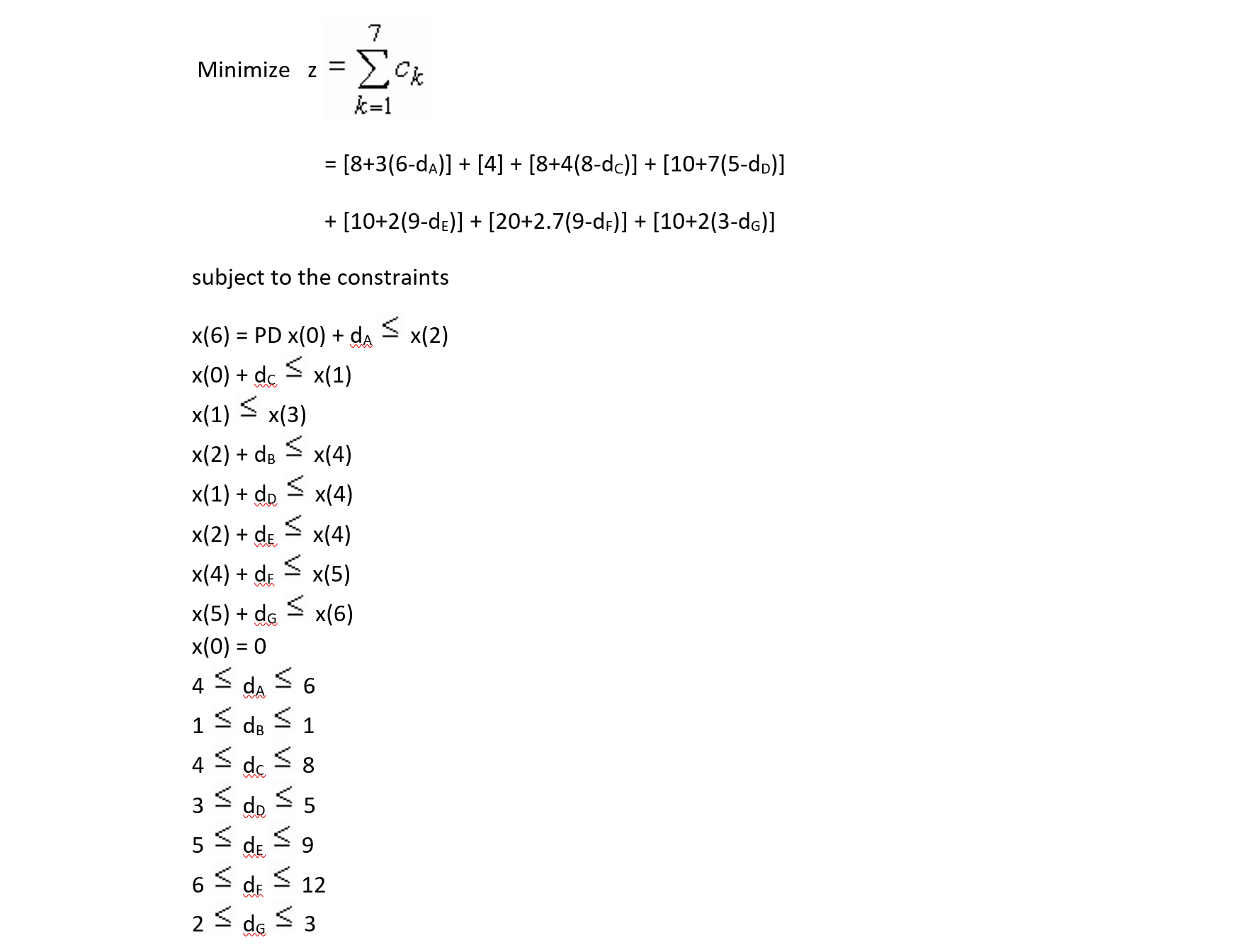
which can be solved for different values of project duration PD using a linear programming algorithm or a network flow algorithm. Note that even with only seven activities, the resulting linear programming problem is fairly large.
11.5 Scheduling in Poorly Structured Problems
The previous discussion of activity scheduling suggested that the general structure of the construction plan was known in advance. With previously defined activities, relationships among activities, and required resources, the scheduling problem could be represented as a mathematical optimization problem. Even in the case in which durations are uncertain, we assumed that the underlying probability distribution of durations is known and applied analytical techniques to investigate schedules.
While these various scheduling techniques have been exceedingly useful, they do not cover the range of scheduling problems encountered in practice. In particular, there are many cases in which costs and durations depend upon other activities due to congestion on the site. In contrast, the scheduling techniques discussed previously assume that durations of activities are generally independent of each other. A second problem stems from the complexity of construction technologies. In the course of resource allocations, numerous additional constraints or objectives may exist that are difficult to represent analytically. For example, different workers may have specialized in one type of activity or another. With greater experience, the work efficiency for particular crews may substantially increase. Unfortunately, representing such effects in the scheduling process can be very difficult. Another case of complexity occurs when activity durations and schedules are negotiated among the different parties in a project so there is no single overall planner.
A practical approach to these types of concerns is to ensure that all schedules are reviewed and modified by experienced project managers before implementation. This manual review permits the incorporation of global constraints or consideration of peculiarities of workers and equipment. Indeed, interactive schedule revision to accommodate resource constraints is often superior to any computer-based heuristic. With improved graphic representations and information availability, human-machine interaction continues to improve as a scheduling procedure.
More generally, the solution procedures for scheduling in these more complicated situations cannot be reduced to mathematical algorithms. A reasonable approach is still a “generate-and-test” cycle for alternative plans and schedules. In this process, a possible schedule is hypothesized or generated. This schedule is tested for feasibility with respect to relevant constraints (such as available resources or time horizons) and desirability with respect to different objectives. Ideally, the process of evaluating an alternative will suggest directions for improvements or identify particular trouble spots. These results are then used in the generation of a new test alternative. This process continues until a satisfactory plan is obtained.
Approaches to automating this type of planning have been proposed based on genetic-algorithms and other AI-based approaches. With AI-scale computing power, such approaches have become feasible computationally. Impediments to their use remain however. The effort involved in identifying and entering all the relevant constraints and parameter values is substantial. They are typically complex to use. And, evaluating the alternatives they generate still involves considerable effort and judgment.
11.6 Human-Machine Interactive Scheduling with Integrated Project Information Technology Systems
Ways to improve planning and scheduling in construction continue to be developed and offered in commercial software packages and services. Most of them include some combination of:
- Integrated graphical displays of plans, schedules, resource loading, bills of quantities, 3D designs, progress and projections of cost and duration to project completion, and more.
- Options to drill down into more detail on all these things
- Sophisticated user interfaces and flexible workflows
- Scheduling, graphics and accounting engines that run in the background to immediately propagate impacts of user entered changes and thus update cost, schedule and project controls data
- Integration with supply chain and materials management functions
- Integration with payroll, payments and invoicing functions
- Integration with corporate business intelligence systems
- Maintenance of interdependencies among sets of activities (e.g. experienced productivity of a particular trade or craft on the project)
Some of these improved and specialized approaches have become broadly accepted in sectors of the industry or in regions of the world. These include:
- Advanced Work Packaging
- Lean Construction
- 4D and 5D BIM
In practice, the boundary between planning, scheduling, control and other project systems is becoming harder to define. One obvious advantage is the elimination of transcription and translation errors and work between different project process management systems. That is generally a good thing, as the integration of the advanced information technology systems required to make this happen has resulted in significant productivity and project performance improvement, as documented by Zhai et al in an article in the ASCE Journal of Construction Engineering and Management published in 2009.
11.7 References
- Bratley, Paul, Bennett L. Fox and Linus E. Schrage, A Guide to Simulation, Springer-Verlag, 1973.
- Elmaghraby, S.E., Activity Networks: Project Planning and Control by Network Models, John Wiley, New York, 1977.
- Jackson, M.J., Computers in Construction Planning and Control, Allen & Unwin, London, 1986.
- Moder, J., C. Phillips and E. Davis, Project Management with CPM, PERT and Precedence Diagramming, Third Edition, Van Nostrand Reinhold Company, 1983.
11.8 Problems
(1) For the project defined in Problem 1 from Chapter 10, suppose that the early, most likely and late time schedules are desired. Assume that the activity durations are approximately normally distributed with means as given in Table 10-16 and the following standard deviations: A: 4; B: 10; C: 1; D: 15; E: 6; F: 12; G: 9; H: 2; I: 4; J: 5; K: 1; L: 12; M: 2; N: 1; O: 5. (a) Find the early, most likely and late time schedules, and (b) estimate the probability that the project requires 25% more time than the expected duration.
(2) For the project defined in Problem 2 from Chapter 10, suppose that the early, most likely and late time schedules are desired. Assume that the activity durations are approximately normally distributed with means as given in Table 10-17 and the following standard deviations: A: 2, B: 2, C: 1, D: 0, E: 0, F: 2; G: 0, H: 0, I: 0, J: 3; K: 0, L: 3; M: 2; N: 1. (a) Find the early, most likely and late time schedules, and (b) estimate the probability that the project requires 25% more time than the expected duration.
(3 to 6)
The time-cost trade-off data corresponding to each of the Problems 1 to 4 (in Chapter 10), respectively are given in the table for the problem (Tables 11-5 to 11-8). Determine the all-crash and the project crash durations and cost based on the early time schedule for the project. Also, suggest a combination of activity durations which will lead to a project completion time equal to three days longer than the project crash time but would result in the (approximately) maximum savings.
(7 to 10)
Develop a project completion time versus cost trade-off curve for the projects in Problems 3 to 6. (Note: a linear programming computer program or more specialized programs can reduce the calculating work involved in these problems!)
(11) Suppose that the project described in Problem 5 from Chapter 10 proceeds normally on an earliest time schedule with all activities scheduled for their normal completion time. However, suppose that activity G requires 20 days rather than the expected 5. What might a project manager do to insure completion of the project by the originally planned completion time?
(12) For the project defined in Problem 1 from Chapter 10, suppose that a Monte Carlo simulation with ten repetitions is desired. Suppose further that the activity durations have a triangular distribution with the following lower and upper bounds: A:4,8; B:4,9, C: 0.5,2; D: 10,20; E: 4,7; F: 7,10; G: 8, 12; H: 2,4; I: 4,7; J: 2,4; K: 2,6; L: 10, 15; M: 2,9; N: 1,4; O: 4,11.
(a) Calculate the value of m for each activity given the upper and lower bounds and the expected duration shown in Table 10-16.
(b) Generate a set of realizations for each activity and calculate the resulting project duration.
(c) Repeat part (b) five times and estimate the mean and standard deviation of the project duration.
(13) Suppose that two variables both have triangular distributions and are correlated. The resulting multi-variable probability density function has a triangular shape. Develop the formula for the conditional distribution of one variable given the corresponding realization of the other variable.
11.9 Footnotes
- See D. G. Malcolm, J.H. Rosenbloom, C.E. Clark, and W. Fazar, “Applications of a Technique for R and D Program Evaluation,” Operations Research, Vol. 7, No. 5, 1959, pp. 646-669. Back
- See M.W. Sasieni, “A Note on PERT Times,” Management Science, Vol. 32, No. 12, p 1986, p. 1652-1653, and T.K. Littlefield and P.H. Randolph, “An Answer to Sasieni’s Question on Pert Times,” Management Science, Vol. 33, No. 10, 1987, pp. 1357-1359. For a general discussion of the Beta distribution, see N.L. Johnson and S. Kotz, Continuous Univariate Distributions-2, John Wiley & Sons, 1970, Chapter 24. Back
- See T. Au, R.M. Shane, and L.A. Hoel, Fundamentals of Systems Engineering – Probabilistic Models, Addison-Wesley Publishing Company, 1972. Back
- See N.L. Johnson and S. Kotz, Distributions in Statistics: Continuous Multivariate Distributions,John Wiley & Sons, New York, 1973. Back
- See, for example, P. Bratley, B. L. Fox and L.E. Schrage, A Guide to Simulation, Springer-Verlag, New York, 1983. Back
- There are exceptions to this rule, though. More workers may also mean additional training burdens and more problems of communication and management. Some activities cannot be easily broken into tasks for numerous individuals; some aspects of computer programming provide notable examples. Indeed, software programming can be so perverse that examples exist of additional workers resulting in slower project completion. See F.P. Brooks, jr. , The Mythical Man-Month, Addison Wesley, Reading, MA 1975. Back
- For a discussion of solution procedures and analogies of the general function time/cost tradeoff problem, see C. Hendrickson and B.N. Janson, “A Common Network Flow Formulation for Several Civil Engineering Problems,” Civil Engineering Systems, Vol. 1, No. 4, 1984, pp. 195-203. Back
- This example was abstracted from work performed in Houston and reported in U. Officer, “Using Accelerated Contracts with Incentive Provisions for Transitway Construction in Houston,” Paper Presented at the January 1986 Transportation Research Board Annual Conference, Washington, D.C. Back
- This description is based on an interactive scheduling system developed at Carnegie Mellon University and described in C. Hendrickson, C. Zozaya-Gorostiza, D. Rehak, E. Baracco-Miller and P. Lim, “An Expert System for Construction Planning,” ASCE Journal of Computing, Vol. 1, No. 4, 1987, pp. 253-269.
