10 Fundamental Scheduling Procedures
10.1 Relevance of Construction Schedules
In addition to assigning dates to project activities, project scheduling is intended to match the resources of equipment, materials and labor with project work tasks over time. Good scheduling can eliminate problems due to production bottlenecks, facilitate the timely procurement of necessary materials, and otherwise ensure the completion of a project as soon as possible. In contrast, poor scheduling can result in considerable waste as laborers and equipment wait for the availability of needed resources or the completion of preceding tasks. Delays in the completion of an entire project due to poor scheduling can also create havoc for owners who are eager to start using the constructed facilities.
Attitudes toward the formal scheduling of projects are often extreme. Many owners require detailed construction schedules to be submitted by contractors as a means of monitoring the work progress. The actual work performed is commonly compared to the schedule to determine if construction is proceeding satisfactorily. After the completion of construction, similar comparisons between the planned schedule and the actual accomplishments may be performed to allocate the liability for project delays due to changes requested by the owner, worker strikes or other unforeseen circumstances.
In contrast to these instances of reliance upon formal schedules, many field supervisors disdain and dislike formal scheduling procedures. In particular, the critical path method of scheduling is commonly required by owners and has been taught in universities for decades, but it is often regarded in the field as irrelevant to actual operations and a time-consuming distraction. The result is “seat-of-the-pants” scheduling that can be good or that can result in grossly inefficient schedules and poor productivity. Progressive construction firms use formal scheduling procedures whenever the complexity of work tasks is high, and the coordination of different workers is required.
Dozens of construction project and work scheduling software packages and cloud-based services are commercially available. Many are specialized for a subsector of the industry (such as homebuilding) or a subset of participants (site superintendents) or for a stage in the supply chain (such as fab shops) or for a specific function (such as BridgitTM for workforce planning). Some have highly simplified interfaces (e.g. Monday | ConstructionTM). Many of these packages interface with other construction project management functions such as payroll, cost and schedule control, materials management, BIM, procurement, portfolio management, etc. Two dominant packages at the time of writing this text are MS ProjectTM and PrimaveraTM. However, problems with the use of formal scheduling methods will continue until managers understand their proper use and limitations.
A basic distinction exists between resource-oriented and time-oriented scheduling techniques. For resource-oriented scheduling, the focus is on using and scheduling particular resources in an effective fashion. For example, the project manager’s main concern on a high-rise building site might be to ensure that cranes are used effectively for moving materials; without effective scheduling in this case, delivery trucks might queue on the ground and workers wait for deliveries on upper floors. For time-oriented scheduling, the emphasis is on determining the completion time of the project given the necessary precedence relationships among activities. Hybrid techniques for resource leveling or resource constrained scheduling in the presence of precedence relationships also exist. Most scheduling software is time-oriented, although virtually all of the programs have the capability to introduce resource constraints.
This chapter will introduce the fundamentals of scheduling methods. Our discussion will generally assume that computer-based scheduling software will be applied, and it will focus on the common core of formal methods implemented by these software packages and services. Even if formal methods are not applied in particular cases, the conceptual framework of formal scheduling methods provides a valuable reference for a manager. Accordingly, examples involving hand calculations will be provided throughout the chapter to facilitate understanding.
10.2 The Critical Path Method
The most widely used scheduling technique is the critical path method (CPM) for scheduling, often referred to as critical path scheduling. This method calculates the minimum completion time for a project along with the possible start and finish times for the project activities. Indeed, many texts and managers regard critical path scheduling as the only usable and practical scheduling procedure. Software packages and services for critical path scheduling are widely available and can efficiently handle projects with thousands of activities.
The critical path itself represents the set or sequence of predecessor/successor activities which will take the longest time to complete. The duration of the critical path is the sum of the activities’ durations along the path. Thus, the critical path can be defined as the longest possible path through the “network” of project activities, as described in Chapter 9. The duration of the critical path represents the minimum time required to complete a project. Any delays along the critical path would imply that additional time would be required to complete the project.
There may be more than one critical path among all the project activities, so completion of the entire project could be delayed by delaying activities along any one of the critical paths. For example, a project consisting of two activities performed in parallel that each require three days would have each activity critical for a completion in three days.
Formally, critical path scheduling assumes that a project has been divided into activities of fixed duration and well-defined predecessor relationships. A predecessor relationship implies that one activity must come before another in the schedule. No resource constraints other than those implied by precedence relationships are recognized in the simplest form of critical path scheduling.
To use critical path scheduling in practice, construction planners often represent a resource constraint by a precedence relation. A constraint is simply a restriction on the options available to a manager, and a resource constraint is a constraint deriving from the limited availability of some resource of equipment, material, space or labor. For example, one of two activities requiring the same piece of equipment might be arbitrarily assumed to precede the other activity. This artificial precedence constraint ensures that the two activities requiring the same resource will not be scheduled at the same time. Also, most critical path scheduling algorithms impose restrictions on the generality of the activity relationships or network geometries which are used. In essence, these restrictions imply that the construction plan can be represented by a network plan in which activities appear as nodes in a network, as in Figure 9-6. Nodes are numbered, and no two nodes can have the same number or designation. Two nodes are introduced to represent the start and completion of the project itself.
The actual computer representation of the project schedule generally consists of a list of activities along with their associated durations, required resources and predecessor activities. Graphical network representations rather than a list are helpful for visualization of the plan and to ensure that mathematical requirements are met. The actual input of the data to a computer program may be accomplished by filling in blanks on a screen menu, dragging and dropping icons, or modifying an existing schedule.
Example 10-1: Formulating a network diagram
Suppose that we wish to form an activity network for a seven-activity project with the following precedences:
| Activity | Predecessors |
| A B C D E F G |
— — A,B C C D D,E |
An activity-on-node representation is shown in Figure 10-1, including project start and finish nodes.
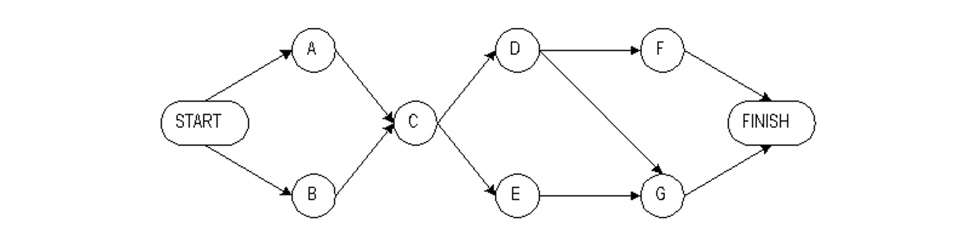
Figure 10-1 An Activity-on-Node Network for Critical Path Scheduling
10.3 Calculations for Critical Path Scheduling
With the background provided by the previous sections, we can formulate critical path scheduling mathematically. We assume that all precedences are of a finish-to-start nature, so that a succeeding activity cannot start until the completion of a preceding activity. In a later section, we present a comparable algorithm for activity-on-node representations with multiple precedence types.
Suppose that our project network has n+1 nodes, the initial event being 0 and the last event being n. Let the time at which node events occur be x1, x2,…., xn, respectively. The start of the project at x0 will be defined as time 0. Nodal event times must be consistent with activity durations, so that an activity’s successor node event time must be larger than an activity’s predecessor node event time plus its duration. For an activity defined as starting from event i and ending at event j, this relationship can be expressed as the inequality constraint, xj xi + Dij where Dij is the duration of activity (i,j). This same expression can be written for every activity and must hold true in any feasible schedule. Mathematically, then, the critical path scheduling problem is to minimize the time of project completion (xn) subject to the constraints that each node completion event cannot occur until each of the predecessor activities have been completed:
Minimize

subject to

This is a linear programming problem since the objective value to be minimized and each of the constraints is a linear equation. [1]
Rather than solving the critical path scheduling problem with a linear programming algorithm (such as the Simplex method), more efficient techniques are available that take advantage of the network structure of the problem. These solution methods are very efficient with respect to the required computations, so that very large networks can be treated even with personal computers. These methods also give some very useful information about possible activity schedules. The programs can compute the earliest and latest possible starting times for each activity which are consistent with completing the project in the shortest possible time. This calculation is of particular interest for activities which are not on the critical path (or paths), since these activities might be slightly delayed or re-scheduled over time as a manager desires without delaying the entire project.
An efficient solution process for critical path scheduling based upon node labeling is shown in Table 10-1. Three algorithms appear in the table. The activity numbering algorithm numbers the nodes (or activities) of the project such that all predecessors of an activity have a lower number. Technically, this algorithm accomplishes a “topological sort” of the activities. The project start node is given number 0.
We define: ES(i) as the earliest start time for activity (and node) i, EF(i) is the earliest finish time for activity (and node) i, LS(i) is the latest start and LF(i) is the latest finish time for activity (and node) i. Table 10-1 shows the relevant calculations for the node numbering algorithm, the forward pass and the backward pass calculations.
TABLE 10-1 Critical Path Scheduling Algorithms (Activity-on-Node Representation)
| Activity Numbering Algorithm |
| Step 1: Give the starting activity number 0. Step 2: Give the next number to any unnumbered activity whose predecessor activities are each already numbered. Repeat Step 2 until all activities are numbered. |
| Forward Pass |
| Step 1: Let ES(0) = 0, D0=0, and EF(0)=0 Step 2: For j = 1,2,3,…,n (where n is the last activity), let ES(j) = maximum {EF(i)} where the maximum is computed over all activities (i) that have j as their successor. Step 3: EF(j) = ES(j) + Dj |
| Backward Pass |
| Step 1: Set EF(n) Step 2: For i = n-1, n-2, …, 0, let LF(i) = minimum {LS(j)} where the minimum is computed over all activities (j) that have i as their predecessor. Step 3: LS(i) = LF(i) – Di |
The forward pass algorithm computes the earliest possible time, ES(j), at which each activity, j, in the network can start. Earliest activity start times are computed as the maximum of the earliest start times plus activity durations for each of the activities immediately preceding an event:
(10.2) ES(j) = maximum {EF(i)}
The earliest finish time of each activity i can be calculated by:
(10.3) EF(i) = ES(i) + Di
Activities are identified in this algorithm by the predecessor activity i and the successor activity j. The algorithm simply requires that each activity in the network should be examined in turn beginning with the project start (activity 0).
The backward pass algorithm computes the latest possible time, LF(i), at which each activity, i, in the network can finish, given the desired completion time of the project. Usually, the desired completion time will be equal to the earliest possible completion time, so that EF(n) = ES(n) for the final activity n (which is assigned duration of 0). The algorithm begins with the final activity and works backwards through the project activities. The latest finish time of activity i is equal to the minimum of the latest start times of its successor activities:
(10.4) LF(i) = minimum {LS(j)}
, where the minimum is computed over all activities (j) that have i as their predecessor.
The latest start time of each activity i can be calculated by:
(10.5) LS(i) = LF(i) – Di
The earliest start and latest finish times for each event are useful pieces of information in developing a project schedule. Events which have equal earliest and latest times lie on the critical path or paths. To avoid delaying the project, all the activities on a critical path should begin as soon as possible, so each critical activity i must be scheduled to begin at the earliest possible start time, ES(i).
Example 10-2: Critical path scheduling calculations
Consider the project defined in Table 10-2.
TABLE 10-2 Precedence Relations and Durations for a Nine Activity Project Example
| Activity | Description | Predecessors | Duration |
| A B C D E F G H I |
Site clearing Removal of trees General excavation Grading general area Excavation for trenches Placing formwork and reinforcement for concrete Installing sewer lines Installing other utilities Pouring concrete |
— — A A B, C B, C D, E D, E F, G |
4 3 8 7 9 12 2 5 6 |
An activity-on-node network representation for this project and its precedence relationships is illustrated in Figure 10-2.
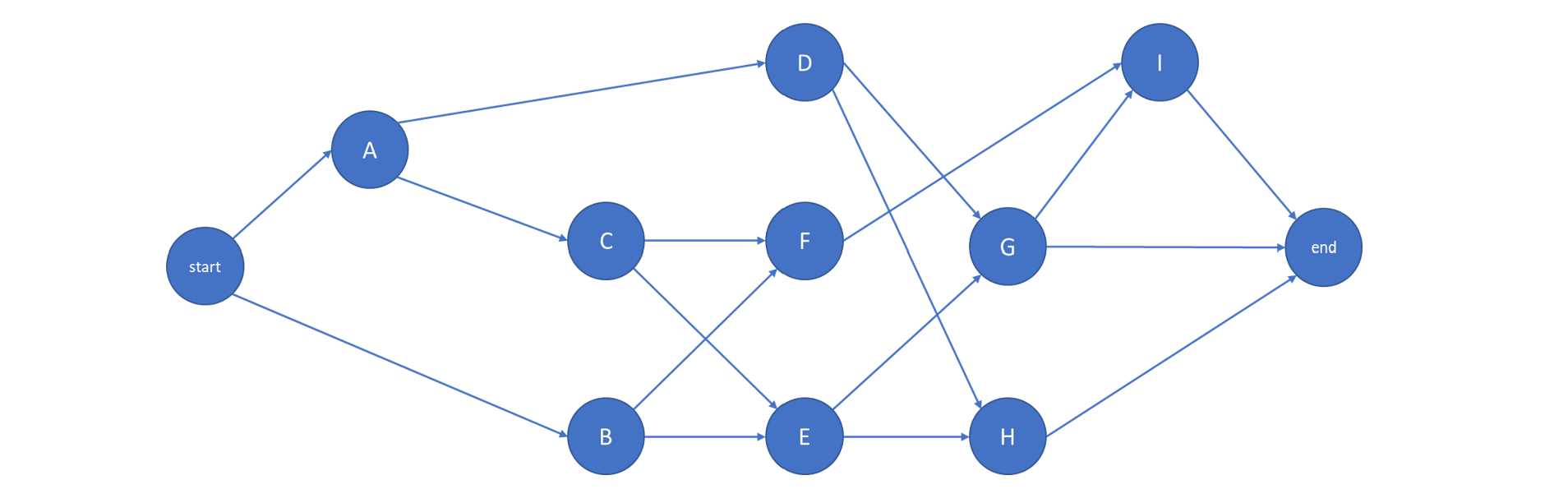
Figure 10-2 A Nine-Activity Project Network
For the network shown in Figure 10-2, the project start is given number 0. Successor activities are numbered as illustrated in Figure 10-3 using the activity numbering algorithm described above. For manually scheduling, hand annotations are adequate, and one option for organizing such annotations is illustrated in Figure 10-3 as well.
Manually solving simple networks like the ones in this chapter is critical to achieving the minimum understanding required for using scheduling and project management software effectively. Concepts addressed in subsequent sections and chapters, such as resource leveling, or schedule crashing only make sense when the fundamental scheduling constraints are understood. Then, the full power of the software can be used.
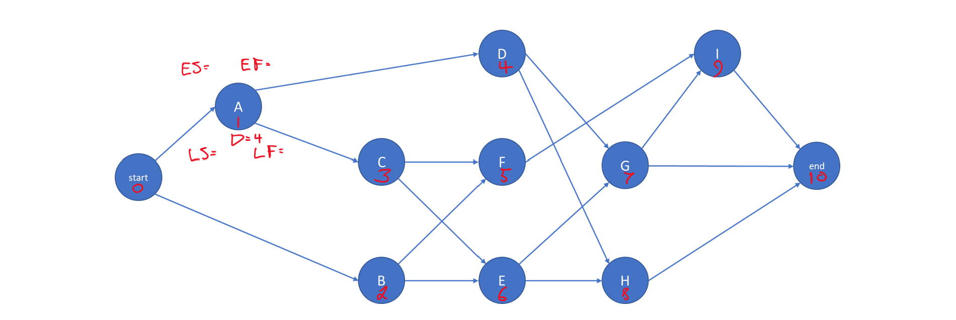
Figure 10-3 A Hand-annotated Nine-Activity Project Network
For the network in Figure 10-3 with activity durations in Table 10-2, the earliest start time calculations proceed as follows:
| Step 1 | E(0) = 0 |
| Step 2 | |
| j = 1 | ES(1) = Max{ES(0) + D0} = Max{ 0 + 0 } = 0 |
| j = 2 | ES(2) = Max{ES(0) + D0} = Max{ 0 + 0 } = 0 |
| j = 3 | ES(3) = Max{ES(1) + D1} = Max{ 0 + 4 } = 4 |
| j = 4 | ES(4) = Max{ES(1) + D1} = Max{ 0 + 4 } = 4 |
| j = 5 | ES(5) = Max{ES(2) + D2; ES(3) + D3} = Max{0 + 3; 4 + 8} = 12 |
| j = 6 | ES(6) = Max{ES(2) + D2; ES(3) + D3} = Max{0 + 3; 4 + 8} = 12 |
| j = 7 | ES(7) = Max{ES(4) + D4; ES(6) + D6} = Max{4 + 7; 12 + 9} = 21 |
| j = 8 | ES(8) = Max{ES(4) + D4; ES(6) + D6} = Max{4 + 7; 12 + 9} = 21 |
| j = 9 | ES(9) = Max{ES(5) + D5; ES(7) + D7} = Max{12 + 12; 21 + 2} = 24 |
| j = 10 | ES(10) = Max{ES(7) + D7; ES(8) + D8; ES(9) + D9}= Max{21 + 2; 21 + 5; 24 + 6} = 30 |
Thus, the minimum time required to complete the project is 30. In this case, each activity had at most three predecessors.
For the “backward pass,” the latest event time calculations are:
| Step 1 | LF(10) = EF(10) = 30 |
| Step 2 | |
| j = 9 | LF(9) = Min {LS(10)} = Min {LF(10) – D10} = Min {30 – 0} = 30 |
| j = 8 | LF(8) = Min {LS(10)} = Min {LF(10) – D10} = Min {30 – 0} = 30 |
| j = 7 | LF(7) = Min {LS(9); LS(10)} = Min {24; 30} = 24 |
| j = 6 | LF(6) = Min {LS(7); LS(8)} = Min {22; 25} = 22 |
| j = 5 | LF(5) = Min {LS(9)} = Min {24} = 24 |
| j = 4 | LF(4) = Min {LS(7); LS(8)} = Min {22; 25} = 22 |
| j = 3 | LF(3) = Min {LS(5); LS(6)} = Min {12; 13} = 12 |
| j = 2 | LF(2) = Min {LS(5); LS(6)} = Min {12; 13} = 12 |
| j = 1 | LF(1) = Min {LS(3); LS(4)} = Min {4; 15} = 4 |
| j = 0 | LF(0) = Min {LS(1); LS(2)} = Min {0; 9} = 0 |
We can see that activities A, C, F and I are on the critical path. Their early starts equal their late starts, their early finishes equal their late finishes, and the comprise the longest path through the network. These results are recorded in Figure 10-4 in the way one might if solving by hand.
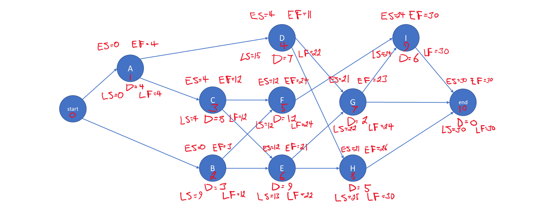
Figure 10-4 A Hand-solved Nine-Activity Project Network
10.4 Activity Float and Schedules
A number of different activity schedules can be developed from the critical path scheduling procedure described in the previous section. An earliest time schedule would be developed by starting each activity as soon as possible, at ES(i). Similarly, a latest time schedule would delay the start of each activity as long as possible but still finish the project in the minimum possible time. This late schedule can be developed by setting each activity’s start time to LS(i).
Activities that have different early and late start times (i.e., ES(i) < LS(i)) can be scheduled to start anytime between ES(i) and LS(i) as shown in Figure 10-6. The concept of float is to use part or all of this allowable range to schedule an activity without delaying the completion of the project. An activity that has the earliest time for its predecessor and successor nodes differing by more than its duration possesses a window in which it can be scheduled. Some float is available in which to schedule this activity. Total float, TF(i), can be calculated as:
(10.6) TF(i) = LS(i) – ES(i)
Or
(10.7) TF(i) = LF(i) – EF(i)
Free float is the amount of time an activity can be delayed without affecting or delaying any of its successors j. Free float, FF(i), can be calculated as:
(10.8) FF(i) = min {ES(j) – EF(i)} for all successors j
Float is a very valuable concept since it represents the scheduling flexibility or “maneuvering room” available to complete particular tasks. Activities on the critical path do not provide any flexibility for scheduling nor leeway in case of problems. For activities with some float, the actual starting time might be chosen to balance work loads over time, to correspond with material deliveries, or to improve the project’s cash flow. Each of these “floats” indicates an amount of flexibility associated with an activity. In all cases, total float equals or exceeds free float. Also, any activity on a critical path has floats equal to zero. The converse of this statement is also true, so any activity which has zero total float can be recognized as being on a critical path. The various categories of activity float are illustrated in Figure 10-6.
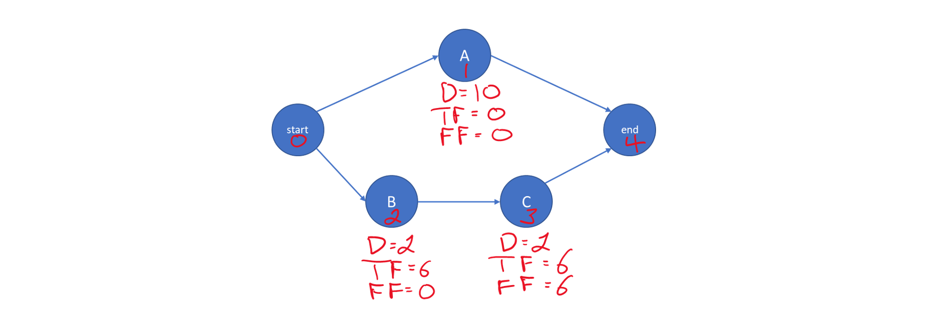
Figure 10-6 Illustration of Activity Float
Example 10-3: Critical path for a fabrication project
As another example of critical path scheduling, consider the seven activities associated with the fabrication of a steel component shown in Table 10-3. Figure 10-7 shows the network diagram and associated with these seven activities. A hand annotated solution for the activity numbering, forward pass and backward pass is also included.
TABLE 10-3 Precedences and Durations for a Seven Activity Project
| Activity | Description | Predecessors | Duration |
| A B C D E F G |
Preliminary design Evaluation of design Contract negotiation Preparation of fabrication plant Final design Fabrication of Product Shipment of Product to owner |
— A — C B, C D, E F |
6 1 8 5 9 12 3 |
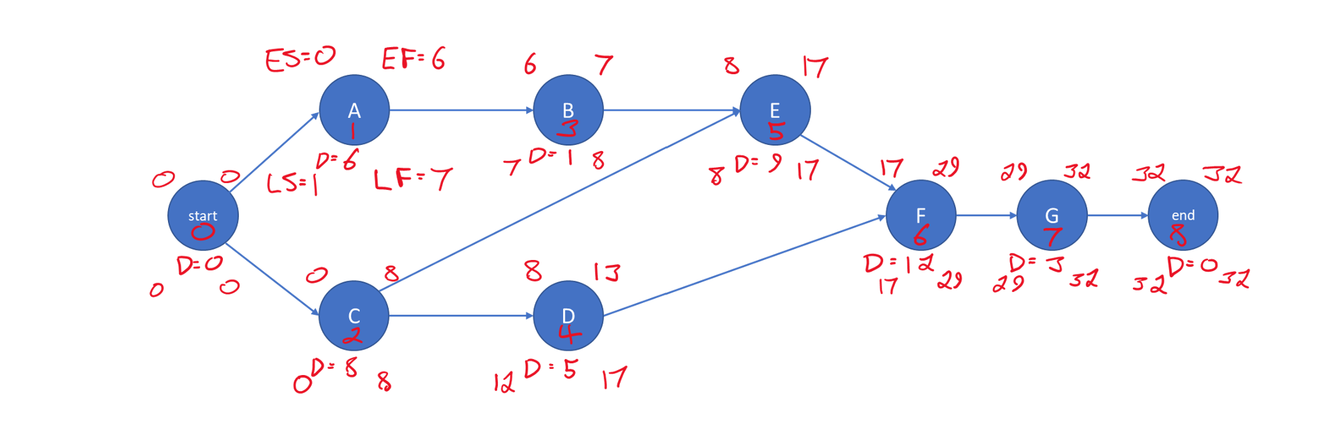
Figure 10-7 Illustration of a Seven Activity Project Network
The minimum completion time for the project is 32 days. Table 10-4 shows the earliest and latest start times for the various activities including the different categories of float. Activities C,E,F,G are on the critical path.
TABLE 10-4 ES, LS, FF and TF for a Seven Activity Project
| Activity | ES (early start) | LS (late start) | FF (free float) | TF (total float) |
| Start | 0 | 0 | 0 | 0 |
| A | 0 | 1 | 0 | 1 |
| B | 6 | 7 | 1 | 1 |
| C | 0 | 0 | 0 | 0 |
| D | 8 | 12 | 4 | 4 |
| E | 8 | 8 | 0 | 0 |
| F | 17 | 17 | 0 | 0 |
| G | 29 | 29 | 0 | 0 |
| End | 32 | 32 | 32 | 32 |
10.5 Presenting Project Schedules
Communicating the project schedule is a vital ingredient in successful project management. A good presentation will greatly ease the manager’s problem of understanding the multitude of activities and their inter-relationships. Moreover, numerous individuals and parties are involved in any project, and they have to understand their assignments. Graphical presentations of project schedules are particularly useful, since it is much easier to comprehend a graphical display of numerous pieces of information than to sift through a large table of numbers. Commercial scheduling software has become quite sophisticated in this regard, and the options are too numerous and rapidly evolving to cover in a text like this, so the basic categories of schedule presentations are simply introduced here.
Network diagrams for projects have already been introduced. These diagrams provide a powerful visualization of the precedences and relationships among the various project activities. They are a basic means of communicating a project plan among the participating planners and project monitors. Project planning is often conducted by producing network representations of greater and greater refinement until the plan is satisfactory.
A useful variation on project network diagrams is to draw a time-scaled network. The activity diagrams shown in the previous section were topological networks in that only the relationship between nodes were of interest. The actual diagram could be distorted in any way desired as long as the connections between nodes were not changed. In time-scaled network diagrams, activities on the network are plotted on a horizontal axis measuring the time since project commencement. Figure 10-8 gives an example of a time-scaled diagram for the seven-activity project in Figure 10-7. In this time-scaled diagram, each node is shown at its earliest possible time. By looking over the horizontal axis, the time at which each activity can begin can be observed. Obviously, this time scaled diagram is produced as a display after activities are initially scheduled by the critical path method. This particular figure is an excellent illustration of why we use software rather than hand drawings.
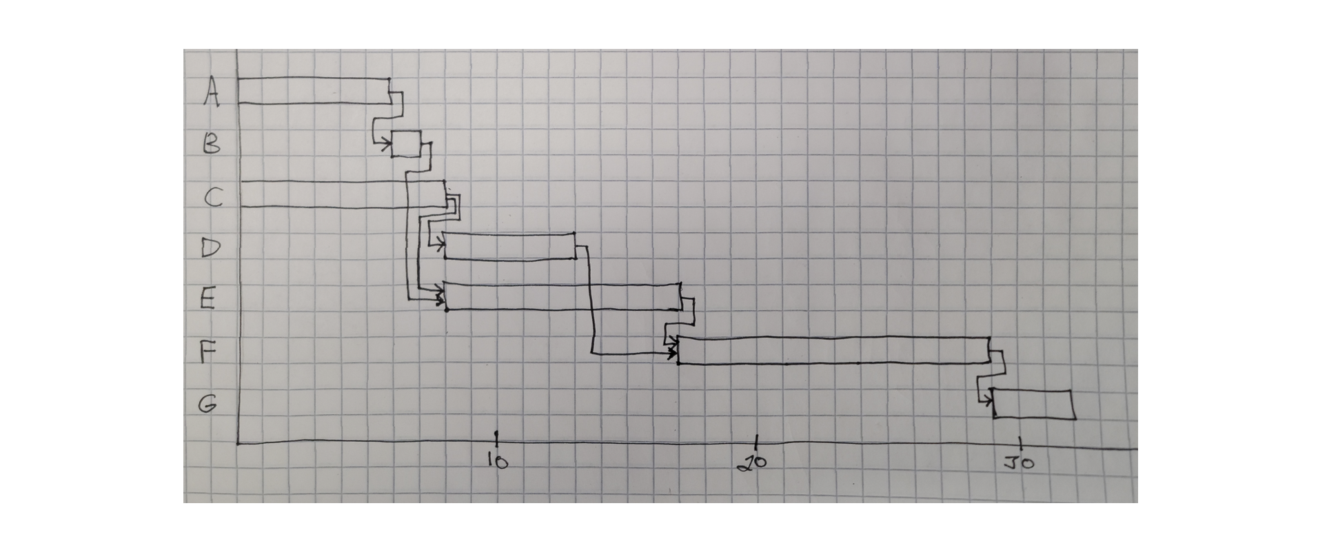
Figure 10-8 Illustration of a Time Scaled Network Diagram with Nine Activities
Another useful graphical representation tool is a bar or Gantt chart illustrating the scheduled time for each activity. The bar chart lists activities and shows their scheduled start, finish and duration. An illustrative bar chart for the nine-activity project appearing in Figure 10-4 is shown in Figure 10-9. Activities are listed in the vertical axis of this figure, while time since project commencement is shown along the horizontal axis. During the course of monitoring a project, useful additions to the basic bar chart include a vertical line to indicate the current time plus small marks to indicate the current state of work on each activity. In Figure 10-9, a hypothetical project state after 4 periods is shown. The small “v” marks on each activity represent the current state of each activity.
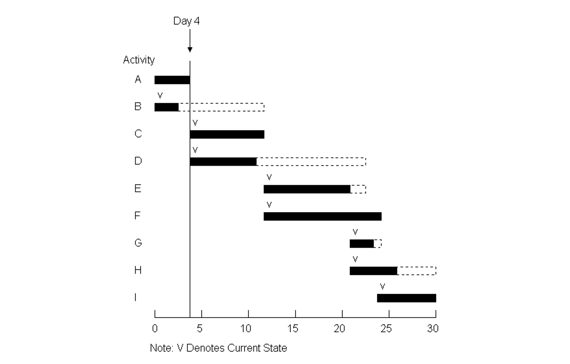
Figure 10-9 An Example Bar Chart for a Nine Activity Project
Bar charts are particularly helpful for communicating the current state and schedule of activities on a project. As such, they have found wide acceptance as a project representation tool in the field. For planning purposes, bar charts are not as useful since they do not indicate the precedence relationships among activities. Thus, a manager must remember or record separately that a change in one activity’s schedule may require changes to successor activities.
Other graphical representations are also useful in project monitoring. Time and activity graphs are extremely useful in portraying the current status of a project as well as the existence of activity float. For example, Figure 10-10 shows two possible schedules for the nine-activity project described in Table 9-1 and shown in the previous figures. The first schedule would occur if each activity was scheduled at its earliest start time, consistent with completion of the project in the minimum possible duration. With this schedule, Figure 10-10 shows the percent of project activity completed versus time. The second schedule in Figure 10-10 is based on latest possible start times for each activity. The horizontal time difference between the two feasible schedules gives an indication of the extent of possible float. If the project goes according to plan, the actual percentage completion at different times should fall between these curves. In practice, a vertical axis representing cash expenditures rather than percent completed is often used in developing a project representation of this type. For this purpose, activity cost estimates are used in preparing a time versus completion graph. Separate “S-curves” may also be prepared for groups of activities on the same graph, such as separate curves for the design, procurement, foundation or particular sub-contractor activities.
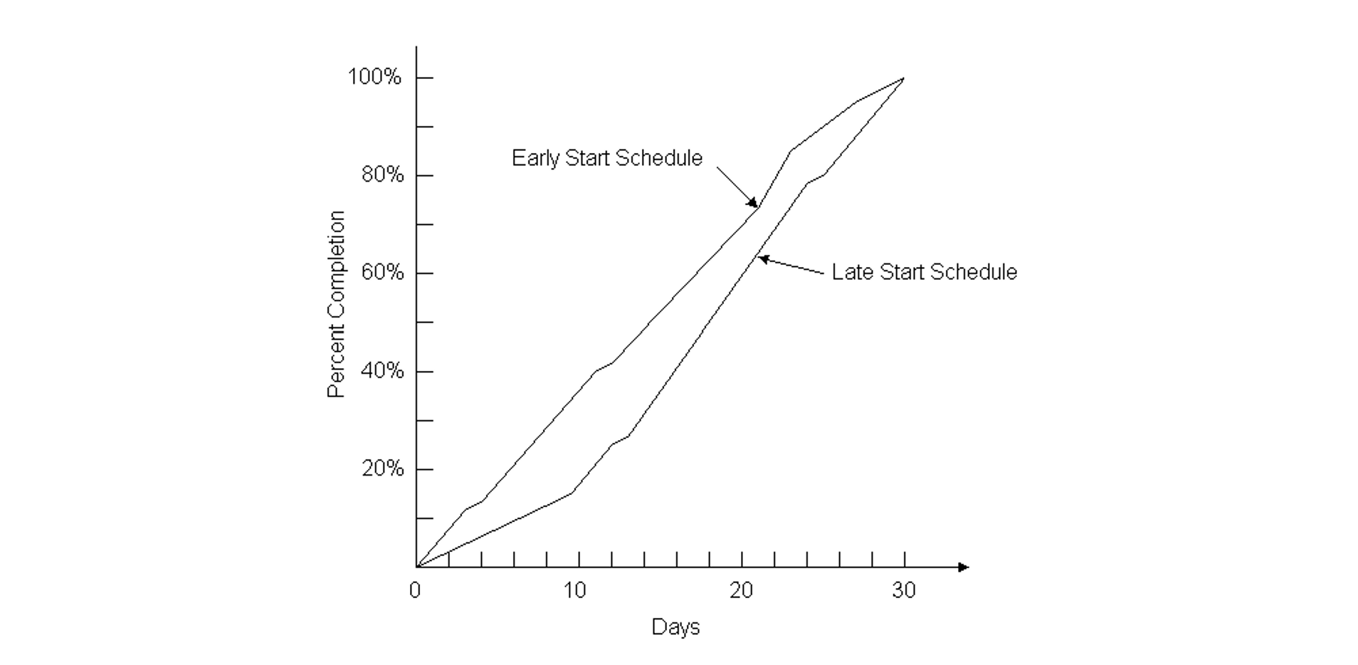
Figure 10-10 Example of Percentage Completion versus Time for Alternative Schedules with a Nine Activity Project
Time versus completion curves are also useful in project monitoring. Not only the history of the project can be indicated, but the future possibilities for earliest and latest start times. For example, Figure 10-11 illustrates a project that is forty percent complete after eight days for the nine-activity example. In this case, the project is well ahead of the original schedule; some activities were completed in less than their expected durations. The possible earliest and latest start time schedules from the current project status are also shown on the figure.
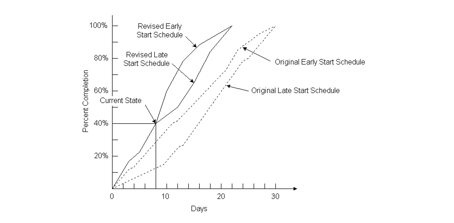
Figure 10-11 Illustration of Actual Percentage Completion versus Time for a Nine Activity Project Underway
Graphs of resource use over time are also of interest to project planners and managers. An example of resource use is shown in Figure 10-12 for the resource of total employment on the site of a project. This graph is prepared by summing the resource requirements for each activity at each time period for a particular project schedule. With limited resources of some kind, graphs of this type can indicate when the competition for a resource is too large to accommodate; in cases of this kind, resource constrained scheduling may be necessary as described in Section 10.9. Even without fixed resource constraints, a scheduler tries to avoid extreme fluctuations in the demand for labor or other resources since these fluctuations typically incur high costs for training, hiring, transportation, and management. Thus, a planner might alter a schedule through the use of available activity floats so as to level or smooth out the demand for resources. Resource graphs such as Figure 10-12 provide an invaluable indication of the potential trouble spots and the success that a scheduler has in avoiding them.
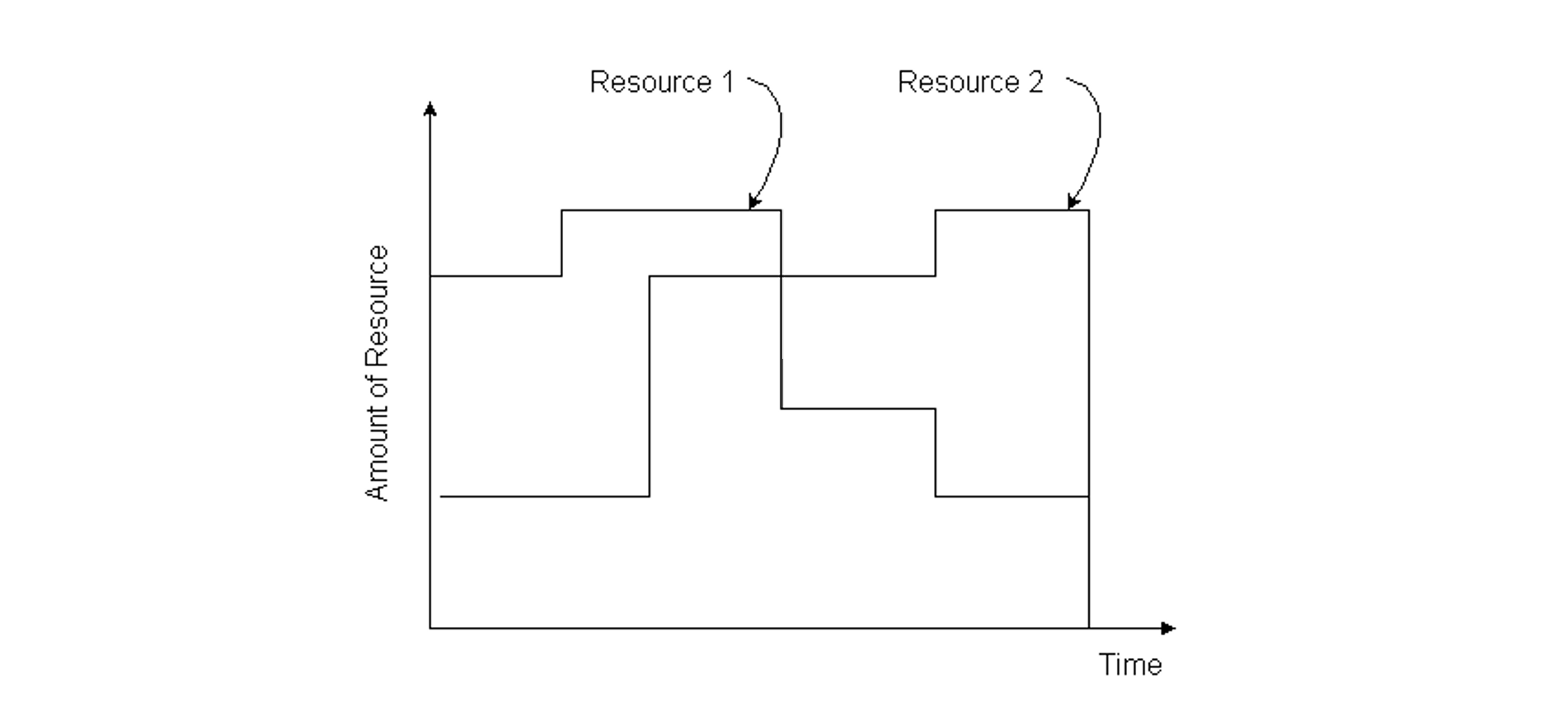
Figure 10-12 Illustration of Resource Use over Time for a Nine Activity Project
A common difficulty with project network diagrams is that too much information is available for easy presentation in a network. A project with, say, five hundred activities, might require the wall space in a room to include the entire diagram using D or E size sheets pinned in a mosaic. In fact, this is not an uncommon sight in the project manager’s office of a large construction project. On a computer display, a typical restriction is that a few dozen activities can be successfully displayed at the same time. The problem of displaying numerous activities becomes particularly acute when accessory information such as activity identifying numbers or phrases, durations and resources are added to the diagram.
One practical solution to this representation problem is to define sets of activities that can be represented together as a single activity. That is, for display purposes, network diagrams can be produced in which one “activity” would represent a number of real sub-activities. For example, an activity such as “foundation design” might be inserted in summary diagrams. In the actual project plan, this one activity could be sub-divided into numerous tasks with their own precedences, durations and other attributes. These sub-groups are sometimes termed fragnets for fragments of the full network. The result of this organization is the possibility of producing diagrams that summarize the entire project as well as detailed representations of particular sets of activities. The hierarchy of diagrams can also be introduced to the production of reports so that summary reports for groups of activities can be produced. Thus, detailed representations of particular activities such as plumbing might be prepared with all other activities either omitted or summarized in larger, aggregate activity representations. Most commercial construction project scheduling and project management software allows for these types of representations. Even if summary reports and diagrams are prepared, the actual scheduling uses detailed activity characteristics, of course.
An example figure of a sub-network appears in Figure 10-13. Summary displays would include only a single node A to represent the set of activities in the sub-network. Note that precedence relationships shown in the master network would have to be interpreted with care, since a particular precedence might be due to an activity that would not commence at the start of activity on the sub-network.
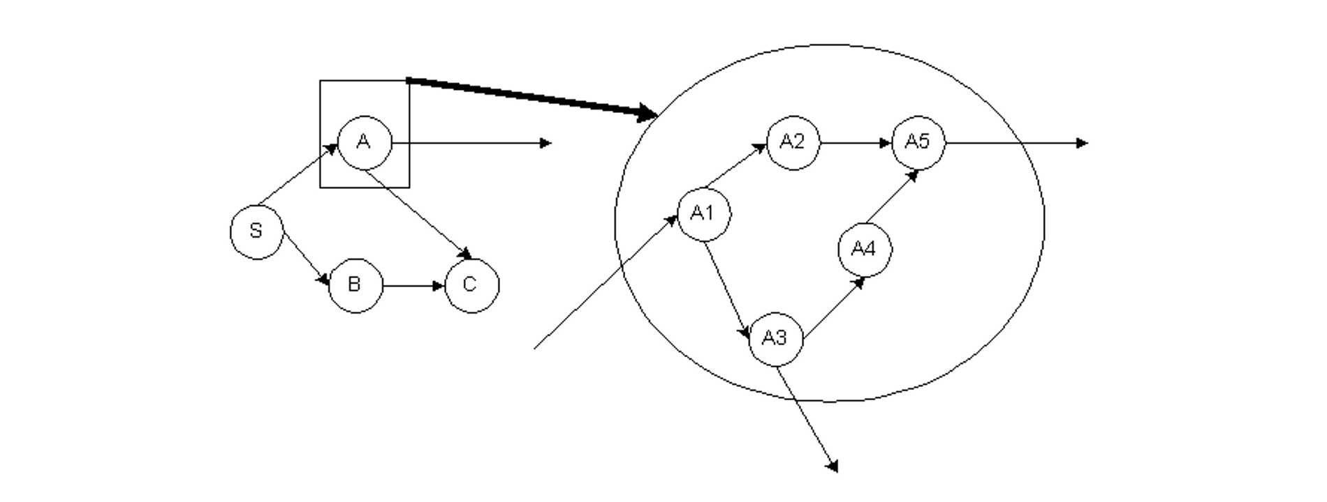
Figure 10-13 Illustration of a Sub-Network in a Summary Diagram
The use of graphical project representations is an important and extremely useful aid to planners and managers. Of course, detailed numerical reports may also be required to check the peculiarities of particular activities. But graphs and diagrams provide an invaluable means of rapidly communicating or understanding a project schedule.
Finally, the scheduling procedure described in Section 10.3 simply counted days from the initial starting point. Scheduling programs typically include several calendar conversion options to provide calendar dates for scheduled work as well as the number of days from the initiation of the project. Such a conversion can be accomplished by establishing a one-to-one correspondence between project dates and calendar dates. For example, project day 2 would be May 4 if the project began at time 0 on May 2 and no holidays intervened. In this calendar conversion, weekends and holidays would be excluded from consideration for scheduling, although the planner might overrule this feature. Also, the number of work shifts or working hours in each day could be defined, to provide consistency with the time units used is estimating activity durations. Project reports and graphs typically use actual calendar days.
10.6 Critical Path Scheduling for Activity-on-Node and with Leads, Lags, and Windows
Building on the critical path scheduling calculations described in the previous sections, some additional capabilities are useful. Desirable extensions include the definition of allowable windows for activities and the introduction of more complicated precedence relationships among activities. For example, a planner may wish to have an activity of removing formwork from a new building component follow the concrete pour by some pre-defined lag period to allow setting. This delay would represent a required gap between the completion of a preceding activity and the start of a successor. The scheduling calculations to accommodate these complications will be described in this section. Again, the standard critical path scheduling assumptions of fixed activity durations and unlimited resource availability will be made here, although these assumptions will be relaxed in later sections.
A capability of many scheduling software packages is to incorporate types of activity interactions in addition to the straightforward predecessor-finish-to-successor-start constraint used in Section 10.3. Incorporation of additional categories of interactions is often called precedence diagramming. [2] For example, it may be the case that installing concrete forms in a foundation trench might begin a few hours after the start of the trench excavation. This would be an example of a start-to-start constraint with a lead: the start of the trench-excavation activity would lead the start of the concrete-form-placement activity by a few hours. Eight separate categories of precedence constraints can be defined, representing greater than (leads) or less than (lags) time constraints for each of four different inter-activity relationships. These relationships are summarized in Table 10-8. Typical precedence relationships would be:
- Direct or finish-to-start leads
The successor activity cannot start until the preceding activity is complete by at least the prescribed lead time (FS). Thus, the start of a successor activity must exceed the finish of the preceding activity by at least FS. - Start-to-start leads
The successor activity cannot start until work on the preceding activity has been underway by at least the prescribed lead time (SS). - Finish-to-finish leads
The successor activity must have at least FF periods of work remaining at the completion of the preceding activity. - Start-to-finish leads
The successor activity must have at least SF periods of work remaining at the start of the preceding activity.
While the eight precedence relationships in Table 10-5 are all possible, the most common precedence relationship is the straightforward direct precedence between the finish of a preceding activity and the start of the successor activity with no required gap (so FS = 0).
TABLE 10-5 Eight Possible Activity Precedence Relationships
| Relationship | Explanation |
| Finish-to-start Lead | Latest Finish of Predecessor Earliest Start of Successor + FS |
| Finish-to-start Lag | Latest Finish of Predecessor Earliest Start of Successor + FS |
| Start-to-start Lead | Earliest Start of Predecessor Earliest Start of Successor + SS |
| Start-to-start Lag | Earliest Start of Predecessor Earliest Start of Successor + SS |
| Finish-to-finish Lead | Latest Finish of Predecessor Earliest Finish of Successor + FF |
| Finish-to-finish Lag | Latest Finish of Predecessor Earliest Finish of Successor + FF |
| Start-to-finish Lead | Earliest Start of Predecessor Earliest Finish of Successor + SF |
| Start-to-finish Lag | Earliest Start of Predecessor Earliest Finish of Successor + SF |
The computations with these lead and lag constraints are somewhat more complicated variations on the basic calculations defined in Table 10-1 for critical path scheduling. Scheduling software computes them automatically.
The possibility of interrupting or splitting activities into two work segments can be particularly important to insure feasible schedules in the case of numerous lead or lag constraints. With activity splitting, an activity is divided into two sub-activities with a possible gap or idle time between work on the two sub-activities. The computations for scheduling treat each sub-activity separately after a split is made. Splitting is performed to reflect available scheduling flexibility or to allow the development of a feasible schedule. For example, splitting may permit scheduling the early finish of a successor activity at a date later than the earliest start of the successor plus its duration. In effect, the successor activity is split into two segments with the later segment scheduled to finish after a particular time. Most commonly, this occurs when a constraint involving the finish time of two activities determines the required finish time of the successor. When this situation occurs, it is advantageous to split the successor activity into two so the first part of the successor activity can start earlier but still finish in accordance with the applicable finish-to-finish constraint.
Finally, the definition of activity windows can be extremely useful. An activity window defines a permissible period in which an activity may be scheduled. To impose a window constraint, a planner could specify an earliest possible start time for an activity (WES) or a latest possible completion time (WLF). Latest possible starts (WLS) and earliest possible finishes (WEF) might also be imposed. In the extreme, a required start time might be insured by setting the earliest and latest window start times equal (WES = WLS). These window constraints would be in addition to the time constraints imposed by precedence relationships among the various project activities. Window constraints are particularly useful in enforcing milestone completion requirements on project activities. For example, a milestone activity may be defined with no duration but a latest possible completion time. Any activities preceding this milestone activity cannot be scheduled for completion after the milestone date. Window constraints are actually a special case of the other precedence constraints summarized above: windows are constraints in which the precedecessor activity is the project start. Thus, an earliest possible start time window (WES) is a start-to-start lead.
Most commercially available computer scheduling software packages include the necessary computational procedures to incorporate windows and many of the various precedence relationships described above. They also include easy to understand graphical representations of these relationships. In the next section, the various computations associated with critical path scheduling with several types of leads, lags and windows are presented.
10.7 Calculations for Scheduling with Leads, Lags and Windows
Table 10-6 contains an algorithmic description of the calculations required for critical path scheduling with leads, lags and windows. This description assumes an activity-on-node project network representation, since this representation is much easier to use with complicated precedence relationships. The possible precedence relationships accommodated by the procedure contained in Table 10-6 are finish-to-start leads, start-to-start leads, finish-to-finish lags and start-to-finish lags. Windows for earliest starts or latest finishes are also accommodated. Incorporating other precedence and window types in a scheduling procedure is also possible as described in Chapter 11. With an activity-on-node representation, we assume that an initiation and a termination activity are included to mark the beginning and end of the project. The set of procedures described in Table 10-6 does not provide for automatic splitting of activities.
TABLE 10-6 Critical Path Scheduling Algorithms with Leads, Lags and Windows
| Activity Numbering Algorithm |
| Step 1: Give the starting activity number 0. Step 2: Give the next number to any unnumbered activity whose predecessor activities are each already numbered. Repeat Step 2 until all activities are numbered. |
| Forward Pass Computations |
| Step 0: Set the earliest start and the earliest finish of the initial activity to zero: (ES(0) = EF(0) = 0). Repeat the following steps for each activity k = 0,1,2,…,m: Step 1: Compute the earliest start time (ES(k)) of activity k: ES(k) = Maximum {0; WES(k) for the earliest start window time, WEF(k) – D(k) for the earliest finish window time; EF(i) + FS(i,k) for each preceding activity with a F-S constraint; ES(i) + SS(i,k) for each preceding activity with a S-S constraint; EF(i) + FF(i,k) – D(k) for each preceding activity with a F-F constraint; ES(i) + SF(i,k) – D(k) for each preceding activity with a S-F constraint.} Step 2: Compute the earliest finish time EF(k) of activity k: EF(k) = ES(k) + D(k). |
| Backward Pass Computations |
| Step 0: Set the latest finish and latest start of the terminal activity to the early start time: LF(m) = LS(m) = ES(m) = EF(m) Repeat the following steps for each activity in reverse order, k = m-1,m-2,…,2,1,0: Step 1: Compute the latest finish time for activity k: LF(k) = Min{ LF(m), WLF(k) for the latest finish window time; WLS(k) + D(k) for the latest start window time; LS(j) – FS(k,j) for each succeeding activity with a F-S constraint; LF(j) – FF(k,j) for each succeeding activity with a FF constraint; LS(j) – SS(k,j) + D(k) for each succeeding activity with a SS constraint; LF(j) – SF(k,j) + D(k) for each succeeding activity with a SF constraint.} Step 2: Compute the latest start time for activity k: LS(k) = LF(k) – D(k) |
The first step in the scheduling algorithm is to sort activities such that no higher numbered activity precedes a lower numbered activity. With numbered activities, durations can be denoted D(k), where k is the number of an activity. Other activity information can also be referenced by the activity number.
The forward pass calculations compute an earliest start time (ES(k)) and an earliest finish time (EF(k)) for each activity in turn (Table 10-6). In computing the earliest start time of an activity k, the earliest start window time (WES), the earliest finish window time (WEF), and each of the various precedence relationships must be considered. Constraints on finish times are included by identifying minimum finish times and then subtracting the activity duration. A default earliest start time of day 0 is also insured for all activities. A second step in the procedure is to identify each activity’s earliest finish time (EF(k)).
The backward pass calculations proceed in a manner very similar to those of the forward pass (Table 10-6). In the backward pass, the latest finish and the latest start times for each activity are calculated. In computing the latest finish time, the latest start time is identified which is consistent with precedence constraints on an activity’s starting time. This computation requires a minimization over applicable window times and all successor activities. A check for a feasible activity schedule can also be imposed at this point: if the late start time is less than the early start time (LS(k) < ES(k)), then the activity schedule is not possible.
The result of the forward and backward pass calculations are the earliest start time, the latest start time, the earliest finish time, and the latest finish time for each activity. The activity float is computed as the latest start time less the earliest start time. Note that window constraints may be instrumental in setting the amount of float, so that activities without any float may either lie on the critical path or be constrained by an allowable window.
To consider the possibility of activity splitting, the various formulas for the forward and backward passes in Table 10-6 must be modified. For example, in considering the possibility of activity splitting due to start-to-start lead (SS), it is important to ensure that the preceding activity has been underway for at least the required lead period. If the preceding activity was split and the first sub-activity was not underway for a sufficiently long period, then the following activity cannot start until the first plus the second sub-activities have been underway for a period equal to SS(i,k). Thus, in setting the earliest start time for an activity, the calculation takes into account the duration of the first subactivity (DA(i)) for preceding activities involving a start-to-start lead. Algebraically, the term in the earliest start time calculation pertaining to start-to-start precedence constraints (ES(i) + SS(i,k)) has two parts with the possibility of activity splitting:
(10.9) ES(i) + SS(i,k)
(10.10) EF(i) – D(i) + SS(i,k) for split preceding activities with DA(i) < SS(i,k)
,where DA(i) is the duration of the first sub-activity of the preceding activity.
The computation of earliest finish time involves similar considerations, except that the finish-to-finish and start-to-finish lag constraints are involved. In this case, a maximization over the following terms is required:
(10.11) EF(k) = Maximum
{ES(k) + D(k),
EF(i) + FF(i,k) for each preceding activity with a FF precedence,
ES(i) + SF(i,k) for each preceding activity with a SF precedence and which is not split,
EF(i) – D(i) + SF(i,k) for each preceding activity with a SF precedence and which is split}
Finally, the necessity to split an activity is also considered. If the earliest possible finish time is greater than the earliest start time plus the activity duration, then the activity must be split.
Another possible extension of the scheduling computations in Table 10-6 would be to include a duration modification capability during the forward and backward passes. This capability would permit alternative work calendars for different activities or for modifications to reflect effects of time of the year on activity durations. For example, the duration of outside work during winter months would be increased. As another example, activities with weekend work permitted might have their weekday durations shortened to reflect weekend work accomplishments.
Example 10-4: Impacts of precedence relationships and windows
To illustrate the impacts of different precedence relationships, consider a project consisting of only two activities in addition to the start and finish. The start is numbered activity 0, the first activity is number 1, the second activity is number 2, and the finish is activity 3. Each activity is assumed to have a duration of five days. With a direct finish-to-start precedence relationship without a lag, the critical path calculations reveal:
ES(0) = 0
ES(1) = 0
EF(1) = ES(1) + D(1) = 0 + 5 = 5
ES(2) = EF(1) + FS(1,2) = 5 + 0 = 5
EF(2) = ES(2) + D(2) = 5 + 5 = 10
ES(3) = EF(2) + FS(2,3) = 10 + 0 = 10 = EF(3)
So the earliest project completion time is ten days.
With a start-to-start precedence constraint with a two-day lead, the scheduling calculations are:
ES(0) = 0
ES(1) = 0
EF(1) = ES(1) + D(1) = 0 + 5 = 5
ES(2) = ES(1) + SS(1,2) = 0 + 2 = 2
EF(2) = ES(2) + D(2) = 2 + 5 = 7
ES(3) = EF(2) + FS(2,3) = 7 + 0 = 7.
In this case, activity 2 can begin two days after the start of activity 1 and proceed in parallel with activity 1. The result is that the project completion date drops from ten days to seven days.
Finally, suppose that a finish-to-finish precedence relationship exists between activity 1 and activity 2 with a two-day lag. The scheduling calculations are:
ES(0) = 0 = EF(0)
ES(1) = EF(0) + FS(0,1) = 0 + 0 = 0
EF(1) = ES(1) + D(1) = 0 + 5 = 5
ES(2) = EF(1) + FF(1,2) – D(2) = 5 + 2 – 5 = 2
EF(2) = ES(2) + D(2) = 2 + 5 = 7
ES(3) = EF(2) + FS(2,3) = 7 + 0 = 7 = EF(3)
In this case, the earliest finish for activity 2 is on day seven to allow the necessary two-day lag from the completion of activity 1. The minimum project completion time is again seven days.
Example 10-5: Scheduling in the presence of leads and windows.
As a second example of the scheduling computations involved in the presence of leads, lags and windows, we shall perform the calculations required for the project shown in Figure 10-14. Start and end activities are included in the project diagram, making a total of eleven activities. The various windows and durations for the activities are summarized in Table 10-7 and the precedence relationships appear in Table 10-8. Only earliest start (WES) and latest finish (WLF) window constraints are included in this example problem. All four types of precedence relationships are included in this project. Note that two activities may have more than one type of precedence relationship at the same time; in this case, activities 2 and 5 have both S-S and F-F precedences. In Figure 10-14, the different precedence relationships are shown by links connecting the activity nodes. The type of precedence relationship is indicated by the beginning or end point of each arrow. For example, start-to-start precedences go from the left portion of the preceding activity to the left portion of the following activity. Application of the activity sorting algorithm (Table 10-6) reveals that the existing activity numbers are appropriate for the critical path algorithm. These activity numbers will be used in the forward and backward pass calculations.
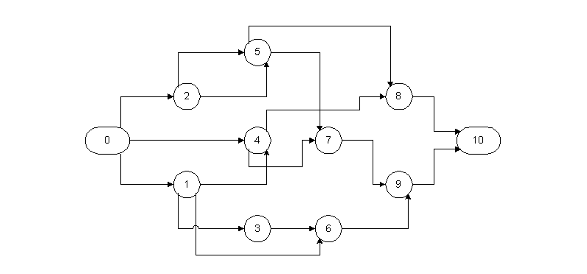
Figure 10-14 Example Project Network with Lead Precedences
TABLE 10-7 Predecessors, Successors, Windows and Durations for an Example Project
| Activity Number | Predecessors | Successors | Earliest Start Window | Latest Finish Window | Activity Duration |
| 0 1 2 3 4 5 6 7 8 9 10 |
— 0 0 1 0 2, 2 1, 3 4, 5 4, 5 6, 7 8, 9 |
1, 2, 4 3, 4, 6 5 6 7, 8 7, 8 9 9 10 10 — |
— — — 2 — — 6 — — — — |
— — — — — 16 16 — — 16 — |
0 2 5 4 3 5 6 2 4 5 0 |
TABLE 10-8 Precedences in a Eleven Activity Project Example
| Predecessor | Successor | Type | Lead |
| 0 0 0 1 1 1 2 2 3 4 4 5 5 6 7 8 9 |
1 2 4 3 4 6 5 5 6 7 8 7 8 9 9 10 10 |
FS FS FS SS SF FS SS FF FS SS FS FS SS FF FS FS FS |
0 0 0 1 1 2 2 2 0 2 0 1 3 4 0 0 0 |
During the forward pass calculations (Table 10-6), the earliest start and earliest finish times are computed for each activity. The relevant calculations are:
ES(0) = EF(0) = 0
ES(1) = Max{0; EF(0) + FS(0,1)} = Max {0; 0 + 0} = 0.
EF(1) = ES(1) + D(1) = 0 + 2 = 2
ES(2) = Max{0; EF(0) + FS(0,1)} = Max{0; 0 + 0} = 0.
EF(2) = ES(2) + D(2) = 0 + 5 = 5
ES(3) = Max{0; WES(3); ES(1) + SS(1,3)} = Max{0; 2; 0 + 1} = 2.
EF(3) = ES(3) + D(3) = 2 + 4 = 6
Note that in the calculation of the earliest start for activity 3, the start was delayed to be consistent with the earliest start time window.
ES(4) = Max{0; ES(0) + FS(0,1); ES(1) + SF(1,4) – D(4)} = Max{0; 0 + 0; 0+1-3} = 0.
EF(4) = ES(4) + D(4) = 0 + 3 = 3
ES(5) = Max{0; ES(2) + SS(2,5); EF(2) + FF(2,5) – D(5)} = Max{0; 0+2; 5+2-5} = 2
EF(5) = ES(5) + D(5) = 2 + 5 = 7
ES(6) = Max{0; WES(6); EF(1) + FS(1,6); EF(3) + FS(3,6)} = Max{0; 6; 2+2; 6+0} = 6
EF(6) = ES(6) + D(6) = 6 + 6 = 12
ES(7) = Max{0; ES(4) + SS(4,7); EF(5) + FS(5,7)} = Max{0; 0+2; 7+1} = 8
EF(7) = ES(7) + D(7) = 8 + 2 = 10
ES(8) = Max{0; EF(4) + FS(4,8); ES(5) + SS(5,8)} = Max{0; 3+0; 2+3} = 5
EF(8) = ES(8) + D(8) = 5 + 4 = 9
ES(9) = Max{0; EF(7) + FS(7,9); EF(6) + FF(6,9) – D(9)} = Max{0; 10+0; 12+4-5} = 11
EF(9) = ES(9) + D(9) = 11 + 5 = 16
ES(10) = Max{0; EF(8) + FS(8,10); EF(9) + FS(9,10)} = Max{0; 9+0; 16+0} = 16
EF(10) = ES(10) + D(10) = 16
As the result of these computations, the earliest project completion time is found to be 16 days.
The backward pass computations result in the latest finish and latest start times for each activity. These calculations are:
LF(10) = LS(10) = ES(10) = EF(10) = 16
LF(9) = Min{WLF(9); LF(10);LS(10) – FS(9,10)} = Min{16;16; 16-0} = 16
LS(9) = LF(9) – D(9) = 16 – 5 = 11
LF(8) = Min{LF(10); LS(10) – FS(8,10)} = Min{16; 16-0} = 16
LS(8) = LF(8) – D(8) = 16 – 4 = 12
LF(7) = Min{LF(10); LS(9) – FS(7,9)} = Min{16; 11-0} = 11
LS(7) = LF(7) – D(7) = 11 – 2 = 9
LF(6) = Min{LF(10); WLF(6); LF(9) – FF(6,9)} = Min{16; 16; 16-4} = 12
LS(6) = LF(6) – D(6) = 12 – 6 = 6
LF(5) = Min{LF(10); WLF(10); LS(7) – FS(5,7); LS(8) – SS(5,8) + D(8)} = Min{16; 16; 9-1; 12-3+4} = 8
LS(5) = LF(5) – D(5) = 8 – 5 = 3
LF(4) = Min{LF(10); LS(8) – FS(4,8); LS(7) – SS(4,7) + D(7)} = Min{16; 12-0; 9-2+2} = 9
LS(4) = LF(4) – D(4) = 9 – 3 = 6
LF(3) = Min{LF(10); LS(6) – FS(3,6)} = Min{16; 6-0} = 6
LS(3) = LF(3) – D(3) = 6 – 4 = 2
LF(2) = Min{LF(10); LF(5) – FF(2,5); LS(5) – SS(2,5) + D(5)} = Min{16; 8-2; 3-2+5} = 6
LS(2) = LF(2) – D(2) = 6 – 5 = 1
LF(1) = Min{LF(10); LS(6) – FS(1,6); LS(3) – SS(1,3) + D(3); Lf(4) – SF(1,4) + D(4)}
LS(1) = LF(1) – D(1) = 2 -2 = 0
LF(0) = Min{LF(10); LS(1) – FS(0,1); LS(2) – FS(0,2); LS(4) – FS(0,4)} = Min{16; 0-0; 1-0; 6-0} = 0
LS(0) = LF(0) – D(0) = 0
The earliest and latest start times for each of the activities are summarized in Table 10-9. Activities without float are 0, 1, 6, 9 and 10. These activities also constitute the critical path in the project. Note that activities 6 and 9 are related by a finish-to-finish precedence with a 4-day lag. Decreasing this lag would result in a reduction in the overall project duration.
TABLE 10-9 Summary of Activity Start and Finish Times for an Example Problem
| Activity | Earliest Start | Latest Start | Float |
| 0 1 2 3 4 5 6 7 8 9 10 |
0 0 0 0 0 2 6 8 5 11 16 |
0 0 1 2 6 3 6 9 12 11 16 |
0 0 1 2 6 1 0 1 7 0 0 |
10.8 Resource Oriented Scheduling
Resource constrained scheduling should be applied whenever there are limited resources available for a project and the competition for these resources among the project activities is keen. In effect, delays are liable to occur in such cases as activities must wait until common resources become available. To the extent that resources are limited and demand for the resource is high, this waiting may be considerable. In turn, the congestion associated with these waits represents increased costs, poor productivity and, in the end, project delays. Schedules made without consideration for such bottlenecks can be completely unrealistic.
Resource constrained scheduling is of particular importance in managing multiple projects with fixed resources of staff or equipment. For example, a design office has an identifiable staff which must be assigned to particular projects and design activities. When the workload is heavy, the designers may fall behind on completing their assignments. Government agencies are particularly prone to the problems of fixed staffing levels, although some flexibility in accomplishing tasks is possible through the mechanism of contracting work to outside firms. Construction activities are less susceptible to this type of problem since it is easier and less costly to hire additional personnel for the (relatively) short duration of a construction project. Overtime or double shift work also provide some flexibility.
Resource oriented scheduling also is appropriate in cases in which unique resources are to be used. For example, scheduling excavation operations when one only excavator is available is simply a process of assigning work tasks or job segments on a day-by-day basis while ensuring that appropriate precedence relationships are maintained. In a fab shop, for example, the key resource constraint may be the number of welding bays or stations. Even with more than one resource, this manual assignment process may be quite adequate. However, a planner should be careful to ensure that necessary precedences are maintained.
Resource constrained scheduling represents a considerable challenge and source of frustration to researchers in mathematics and operations research. While algorithms for optimal solution of the resource constrained problem exist, they are generally too computationally expensive to be practical for all but small networks (of less than about 100 nodes). [5] The difficulty of the resource constrained project scheduling problem arises from the combinatorial explosion of different resource assignments which can be made and the fact that the decision variables are integer values representing all-or-nothing assignments of a particular resource to a particular activity. In contrast, simple critical path scheduling deals with continuous time variables. Construction projects typically involve many activities, so optimal solution techniques for resource allocation are not practical.
One possible simplification of the resource-oriented scheduling problem is to ignore precedence relationships. In some applications, it may be impossible or unnecessary to consider precedence constraints among activities. In these cases, the focus of scheduling is usually on efficient utilization of project resources. To ensure minimum cost and delay, a project manager attempts to minimize the amount of time that resources are unused and to minimize the waiting time for scarce resources. This resource-oriented scheduling is often formalized as a problem of “job shop” (or fab shop) scheduling in which numerous tasks are to be scheduled for completion and a variety of discrete resources need to perform operations to complete the tasks. Reflecting the original orientation towards manufacturing applications, tasks are usually referred to as “jobs” and resources to be scheduled are designated “machines.” In the provision of constructed facilities, an analogy would be an architectural/engineering design office in which numerous design related tasks are to be accomplished by individual professionals in different departments. The scheduling problem is to ensure efficient use of the individual professionals (i.e. the resources) and to complete specific tasks in a timely manner.
The simplest form of resource-oriented scheduling is a reservation system for particular resources. In this case, competing activities or users of a resource pre-arrange use of the resource for a particular time period. Since the resource assignment is known in advance, other users of the resource can schedule their activities more effectively. The result is less waiting or “queuing” for a resource. Online reservation systems (including meeting room reservation systems in companies) are useful for this. It is also possible to impose a preference system within the reservation process so that high-priority activities can be accommodated directly.
In the more general case of multiple resources and specialized tasks, practical resource constrained scheduling procedures rely on heuristic (“rule-of-thumb”) procedures to develop good but not necessarily optimal schedules. While this is the occasion for considerable anguish among researchers, the heuristic methods will typically give fairly good results. An example heuristic method is provided in the next section. Manual methods in which a human scheduler revises a critical path schedule in light of resource constraints can also work relatively well. Given that much of the data and the network representation used in forming a project schedule are uncertain, the results of applying heuristic procedures may be quite adequate in practice.
Example 10-6: A Reservation System [6]
A construction project for a high-rise building complex in New York City was severely limited in the space available for staging materials for hauling up the building. On the four-building site, thirty-eight separate cranes and elevators were available, but the number of movements of people, materials and equipment was expected to keep the equipment very busy. With numerous sub-contractors desiring the use of this equipment, the potential for delays and waiting in the limited staging area was considerable. By implementing an online crane reservation system, these problems were nearly entirely avoided. Times were available on a first-come, first-served basis (i.e. first call, first choice of available slots). Penalties were imposed for making an unused reservation. The reservation system permitted rapid modification and updating of information as well as the provision of standard reservation schedules to be distributed (pushed) to all participants automatically.
Example 10-7: Heuristic (“rule-of-thumb”) Resource Allocation
Suppose that a project manager has eleven pipe sections of a pipeline for which necessary support structures and materials are available in a particular week. To work on these eleven pipe sections, five crews are available. The allocation problem is to assign the crews to the eleven pipe sections. This allocation would consist of a list of pipe sections allocated to each crew for work plus a recommendation on the appropriate sequence to undertake the work. The project manager might make assignments to minimize completion time, to ensure continuous work on the pipeline (so that one section on a pipeline run is not left incomplete), to reduce travel time between pipe sections, to avoid congestion among the different crews, and to balance the workload among the crews. Numerous trial solutions could be rapidly generated, especially with the aid of spreadsheet software. For example, if the nine sections had estimated work durations for each of the fire crews as shown in Table 10-10, then the allocations shown in Figure 10-15 would result in a minimum completion time.
TABLE 10-10 Estimated Required Time for Each Work Task in a Resource Allocation Problem
| Section | Work Duration |
| A B C D E F G H I J K |
9 9 8 8 7 7 6 6 5 5 5 |
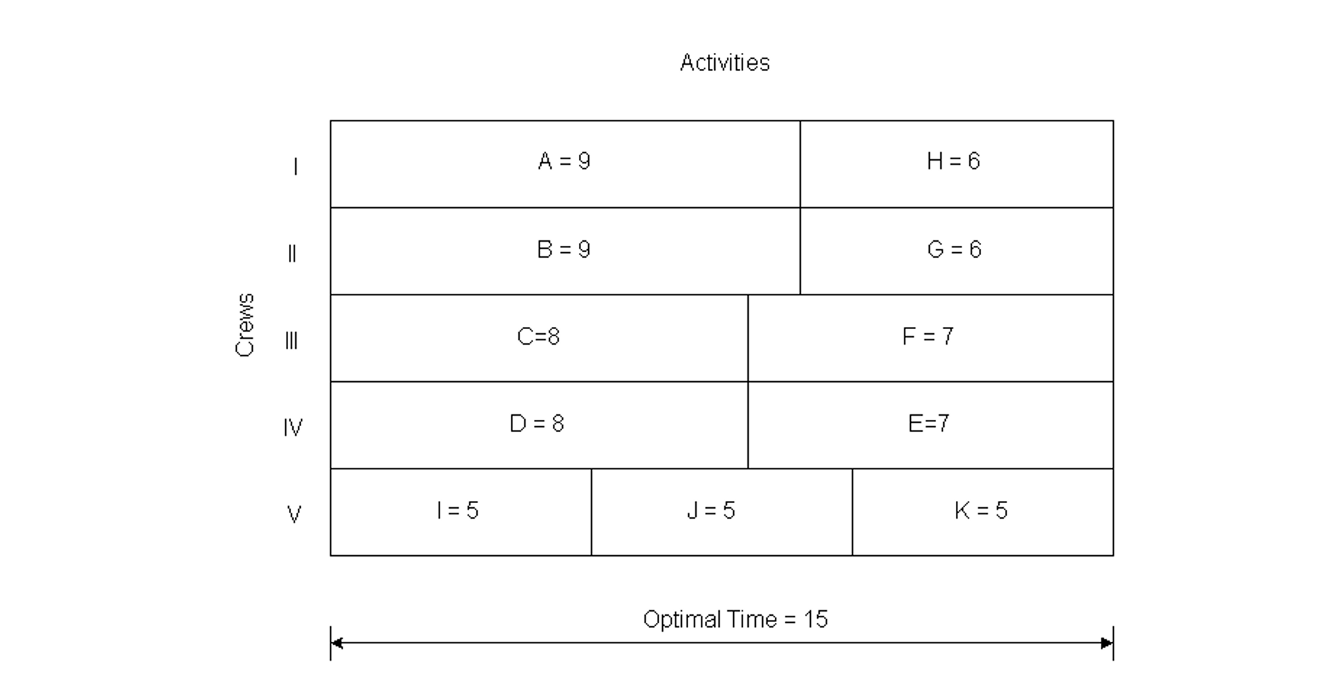
Figure 10-15 Example Allocation of Crews to Work Tasks
Example 10-8: Algorithms for Resource Allocation with Bottleneck Resources
In the previous example, suppose that a mathematical model and solution was desired. For this purpose, we define a binary (i.e. 0 or 1 valued) decision variable for each pipe section and crew, xij, where xij = 1 implies that section i was assigned to crew j and xij = 0 implied that section i was not assigned to crew j. The time required to complete each section is ti. The overall time to complete the nine sections is denoted z.

subject to the constraints:

for each section i,
xij is 0 or 1
where the constraints simply ensure that each section is assigned to one and only one crew. A modification permits a more conventional mathematical formulation, resulting in a generalized bottleneck assignment problem:
Minimize z
subject to the constraints:

for each crew j
 for each section i
xij is 0 or 1
This problem can be solved as an integer programming problem, although at considerable computational expense. A common extension to this problem would occur with differential productivities for each crew, so that the time to complete an activity, tij, would be defined for each crew. Another modification to this problem would substitute a cost factor, cj, for the time factor, tj, and attempt to minimize overall costs rather than completion time.
In “Assignment and Allocation Optimization of Partially Multiskilled Workforce,” in the Journal of Construction Engineering and management, Gomar, Haas, and Morton present an extension of the preceding type of problem to large projects with some percent of multi-skilled craft workers. The workers are the constrained resources.
10.9 Scheduling with Resource Constraints and Precedences
The previous section outlined resource-oriented approaches to the scheduling problem. In this section, we shall review some general approaches to integrating both concerns in scheduling.
Two problems arise in developing a resource constrained project schedule. First, it is not necessarily the case that a critical path schedule is feasible. Because one or more resources might be needed by numerous activities, it can easily be the case that the shortest project duration identified by the critical path scheduling calculation is impossible. The difficulty arises because critical path scheduling assumes that no resource availability problems or bottlenecks will arise. Finding a feasible or possible schedule is the first problem in resource constrained scheduling. Of course, there may be numerous possible schedules which conform with time and resource constraints. As a second problem, it is also desirable to determine schedules which have low costs or, ideally, the lowest cost.
Numerous heuristic methods have been suggested for resource constrained scheduling. Many begin from critical path schedules which are modified in light of the resource constraints. Others begin in the opposite fashion by introducing resource constraints and then imposing precedence constraints on the activities. Still others begin with a ranking or classification of activities into priority groups for special attention in scheduling. [7] One type of heuristic may be better than another for different types of problems. Certainly, projects in which only an occasional resource constraint exists might be best scheduled starting from a critical path schedule. At the other extreme, projects with numerous important resource constraints might be best scheduled by considering critical resources first. A mixed approach would be to proceed simultaneously considering precedence and resource constraints.
A simple modification to critical path scheduling has been shown to be effective for a number of scheduling problems and is simple to implement. For this heuristic procedure, critical path scheduling is applied initially. The result is the familiar set of possible early and late start times for each activity. Scheduling each activity to begin at its earliest possible start time may result in more than one activity requiring a particular resource at the same time. Hence, the initial schedule may not be feasible. The heuristic proceeds by identifying cases in which activities compete for a resource and selecting one activity to proceed. The start time of other activities are then shifted later in time. A simple rule for choosing which activity has priority is to select the activity with the earliest CPM late start time (calculated as LS(i,j) = L(j)-Dij) among those activities which are both feasible (in that all their precedence requirements are satisfied) and competing for the resource. This decision rule is applied from the start of the project until the end for each type of resource in turn.
The order in which resources are considered in this scheduling process may influence the ultimate schedule. A good heuristic to employ in deciding the order in which resources are to be considered is to consider more important resources first. More important resources are those that have high costs or that are likely to represent an important bottleneck for project completion. Once important resources are scheduled, other resource allocations tend to be much easier. The resulting scheduling procedure is described in Table 10-11.
The late start time heuristic described in Table 10-11 is only one of many possible scheduling rules. It has the advantage of giving priority to activities which must start sooner to finish the project on time. However, it is myopic in that it doesn’t consider trade-offs among resource types nor the changes in the late start time that will be occurring as activities are shifted later in time. More complicated rules can be devised to incorporate broader knowledge of the project schedule. These complicated rules require greater computational effort and may or may not result in scheduling improvements in the end.
Possibly hundreds of academic journal articles have been published that define and evaluate variations on resource constrained scheduling, particularly related to CPM schedules. Many of the variations proposed have been implemented in commercial scheduling software packages as functions that can be applied for resource constraints or resource levelling. They can be explored almost endlessly. One such variation is described in a later section here.
TABLE 10-11 A Resource-Oriented Scheduling Procedure
| Step 1:
Rank all resources from the most important to the least important, and number the resources i = 1,2,3,…,m. Step 2: Set the scheduled start time for each activity to the earliest start time. For each resource i = 1,2,3,…,m in turn: Step 3: Start at the project beginning, so set t = 0. Step 4: Compute the demand for resource i at time t by summing up the requirements for resource i for all activities scheduled to be underway at time t. If demand for resource i in time t is greater than the resource availability, then select the activity with the greatest late start time requiring resource i at time t, and shift its scheduled start time to time t+1. Repeat Step 4 until the resource constraint at time t for resource i is satisfied. Step 5: Repeat step 4 for each project period in turn, setting t = t+1. |
Example 10-9: Resource constrained scheduling with nine activities.
As an example of resource constrained scheduling, we shall re-examine the nine-activity project discussed in Section 10.3. To begin with, suppose that four workers and two pieces of equipment such as backhoes are available for the project. The required resources for each of the nine project activities are summarized in Table 10-12. Graphs of resource requirements over the 30-day project duration are shown in Figure 10-16. Equipment availability in this schedule is not a problem. However, on two occasions, more than the four available workers are scheduled for work. Thus, the existing project schedule is infeasible and should be altered.
TABLE 10-12 Resources Required and Starting Times for a Nine Activity Project
| Activity | Workers Required | Equipment Required | Earliest Start Time | Latest Start Time | Duration |
| A B C D E F G H I |
2 2 2 2 2 2 2 2 4 |
0 1 1 1 1 0 1 1 1 |
0 0 4 4 12 12 21 21 24 |
0 9 4 15 13 12 22 25 24 |
4 3 8 7 9 12 2 5 6 |
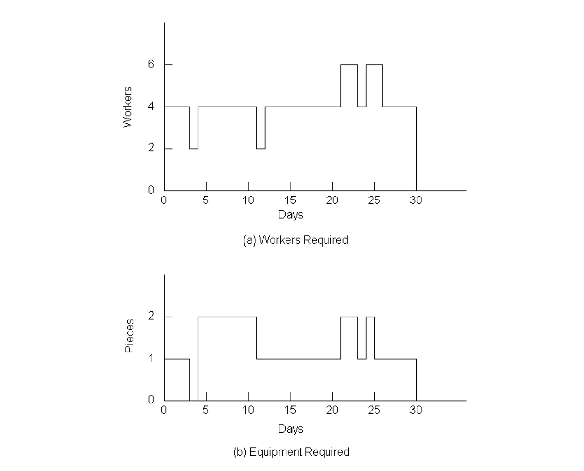
Figure 10-16 Resources Required over Time for Nine Activity Project: Schedule I
The first resource problem occurs on day 21 when activity F is underway and activities G and H are scheduled to start. Applying the latest start time heuristic to decide which activity should start, the manager should re-schedule activity H since it has a later value of LS(i,j), i.e., day 25 versus day 22 as seen in Table 10-12. Two workers become available on day 23 after the completion of activity G. Since activity H is the only activity which is feasible at that time, it is scheduled to begin. Two workers also become available on day 24 at the completion of activity F. At this point, activity I is available for starting. If possible, it would be scheduled to begin with only two workers until the completion of activity H on day 28. If all 4 workers were definitely required, then activity I would be scheduled to begin on day 28. In this latter case, the project duration would be 34 days, representing a 4 day increase due to the limited number of workers available.
Example 10-10: Additional resource constraints.
As another example, suppose that only one piece of equipment was available for the project. As seen in Figure 10-16, the original schedule would have to be significantly modified in this case. Application of the resource constrained scheduling heuristic proceeds as follows as applied to the original project schedule:
-
- On day 4, activities D and C are both scheduled to begin. Since activity D has a larger value of late start time, it should be re-scheduled.
- On day 12, activities D and E are available for starting. Again based on a later value of late start time (15 versus 13), activity D is deferred.
- On day 21, activity E is completed. At this point, activity D is the only feasible activity and it is scheduled for starting.
- On day 28, the planner can start either activity G or activity H. Based on the later start time heuristic, activity G is chosen to start.
- On completion of activity G at day 30, activity H is scheduled to begin.
The resulting profile of resource use is shown in Figure 10-17. Note that activities F and I were not considered in applying the heuristic since these activities did not require the special equipment being considered. In the figure, activity I is scheduled after the completion of activity H due to the requirement of 4 workers for this activity. As a result, the project duration has increased to 41 days. During much of this time, all four workers are not assigned to an activity. At this point, a prudent planner would consider whether or not it would be cost effective to obtain an additional piece of equipment for the project.
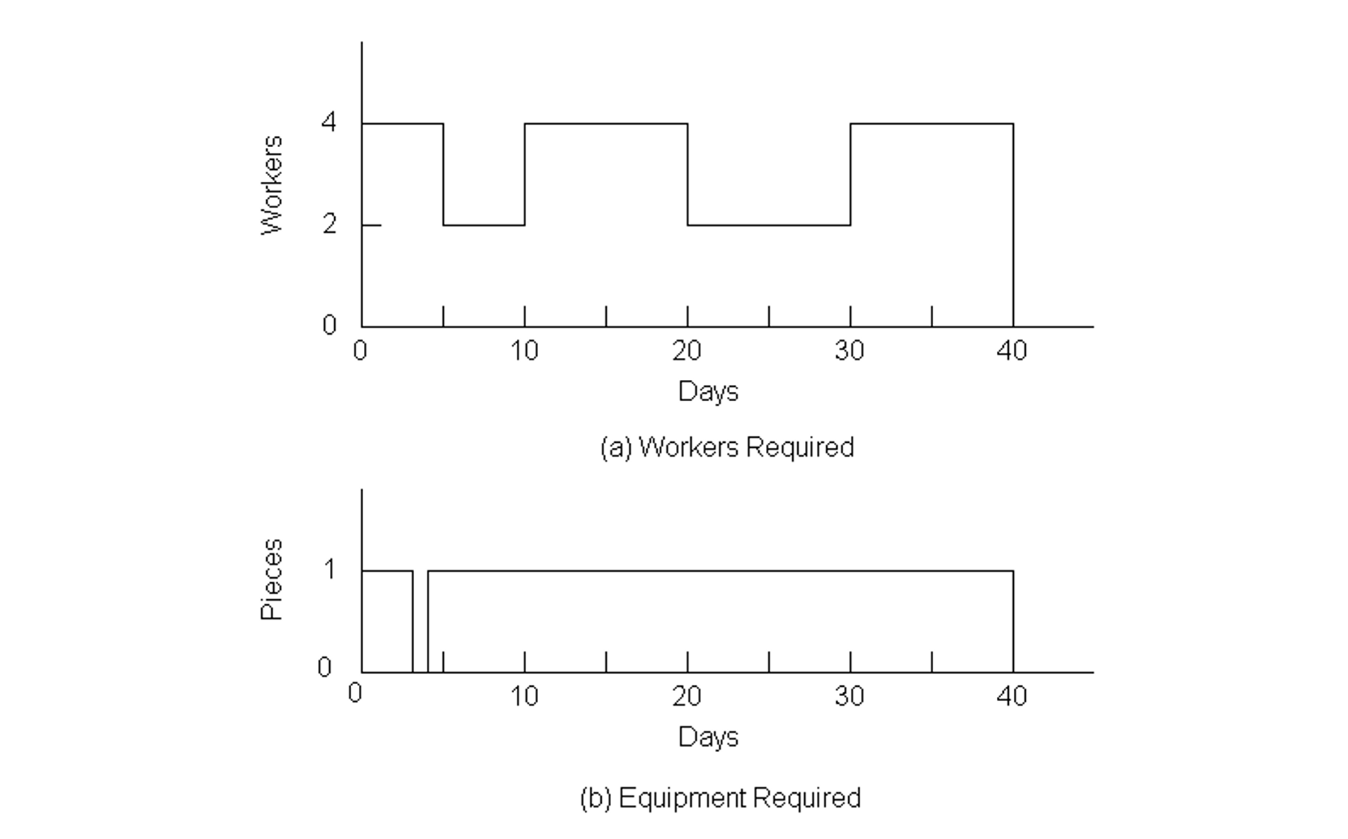
Figure 10-17 Resources Required over Time for Nine Activity Project: Schedule II
10.10 Scheduling Loops
In practice, large, well managed projects adjust their schedules at multiple frequencies depending on the stage and type of work. These frequencies of rescheduling act as nested management control loops. They include:
Critical Path Method (CPM) scheduling, as explained in this chapter:
- A CPM master schedule is typically submitted to the owner by the general contractor prior to project commencement. It may be comprised of many merged subcontractor schedules that meet owner or general contractor-imposed milestones and windows (described in section 10.6). It may have nested networks resulting in levels of the schedule (as described in section 10.5), and it may include many hundreds of resource loaded activities.
- Frequency of updating such a schedule is typically every one to three months on a large project.
Short interval planning or “look-ahead scheduling”:
- Frequency of updating these schedules is typically weekly, by convening weekly meetings between the project manager and key project participants (subcontractors, suppliers, etc.)
- Participants review recently completed, underway, and upcoming activities. They monitor progress and analyze delay causes. They consider what activities are planned to be done according to the master CPM schedule, and which planned activities can be done, based on an assessment of available workers, equipment, materials and information.
- Then, they set goals for the next 5-15 work-days in what are called look-ahead schedules. Such schedules also allocate resources, such as cranes, major equipment, and key crews.
“Toolbox” meetings:
- Every day, foremen on the project should meet with their crew (at the toolboxes) to discuss: (1) the work planned for the day, (2) the availability of materials, equipment, tools and information required, and (3) how to do the work safely. Such meetings are critical for communication, which leads to safe and productive work.
It can be seen that in practice, planning and scheduling on any particular well managed project uses elements of all the methods described in this and the previous chapter in a way that is appropriate for that project.
10.11 References
- Au, T. Introduction to Systems Engineering–Deterministic Models, Addison-Wesley, Reading, MA, 1973, Chapter 8.
- Baker, K., An Introduction to Sequencing and Scheduling, John Wiley, 1974.
- Jackson, M.J., Computers in Construction Planning and Control, Allen & Unwin, 1986.
- Moder, J., C. Phillips and E. Davis, Project Management with CPM, PERT and Precedence Diagramming, Van Nostrand Reinhold Company, Third Edition,1983.
- Willis, E. M., Scheduling Construction Projects, John Wiley & Sons, 1986.
10.12 Problems
(1 to 4) Construct an activity-on-node network from the precedence relationships of activities in the project given in the table for the problem, Tables 10-16 to 10-19.
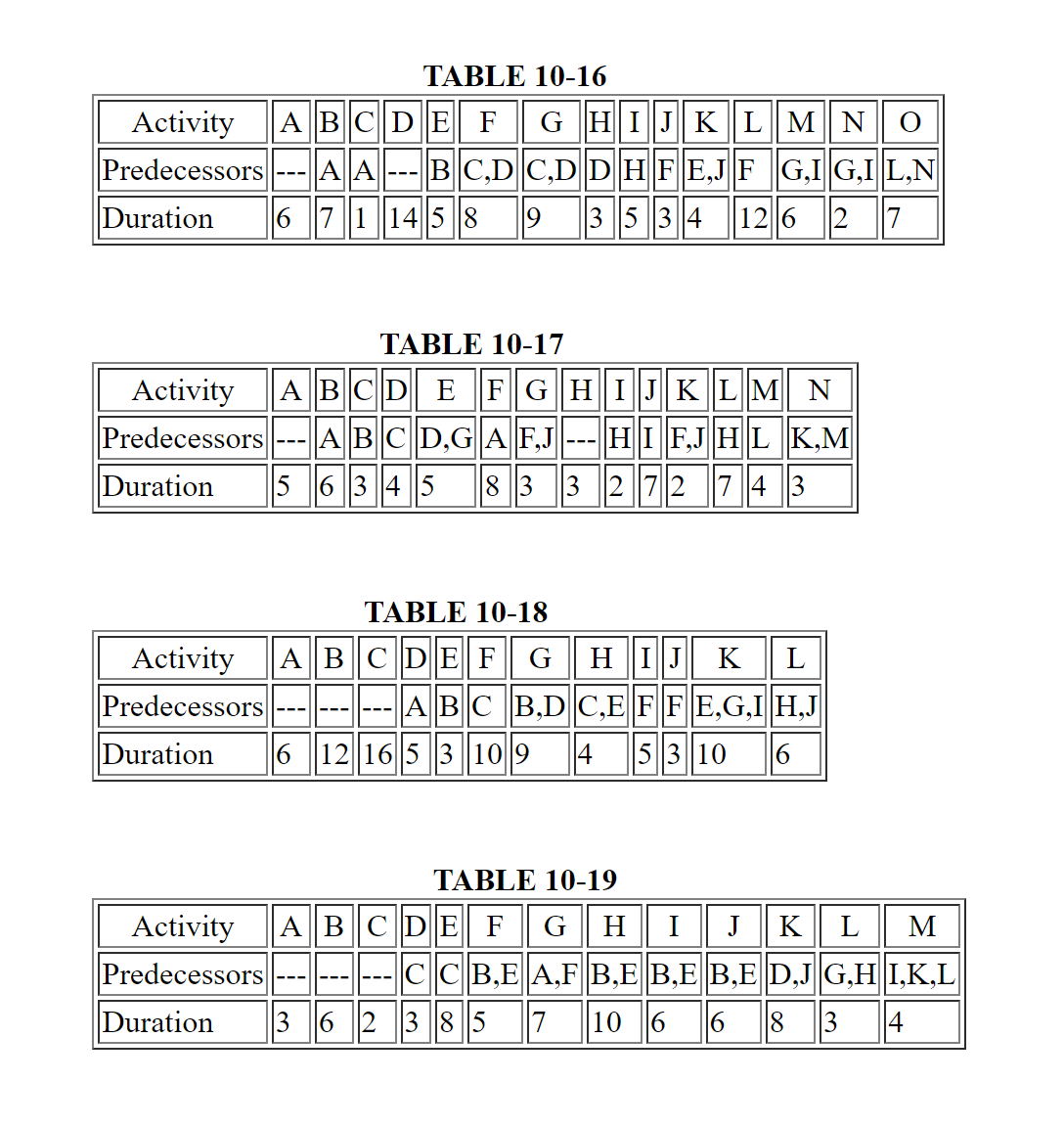
(5 to 8) Determine the critical path and all slacks for the projects in Tables 10-16 to 10-19.
(9) Suppose that the precedence relationships for Problem 1 in Table 10-16 are all direct finish-to-start relationships with no lags except for the following:
-
- B to E: S-S with a lag of 2.
- D to H: F-F with a lag of 3.
- F to L: S-S with a lag of 2.
- G to N: S-S with a lag of 1.
- G to M: S-S with a lag of 2.
Formulate an activity-on-node network representation and recompute the critical path with these precedence relationships.
(10) Suppose that the precedence relationships for Problem 2 in Table 10-17 are all direct finish-to-start relationships with no lags except for the following:
-
- C to D: S-S with a lag of 1
- D to E: F-F with a lag of 3
- A to F: S-S with a lag of 2
- H to I: F-F with a lag of 4
- L to M: S-S with a lag of 1
Formulate an activity-on-node network representation and recompute the critical path with these precedence relationships.
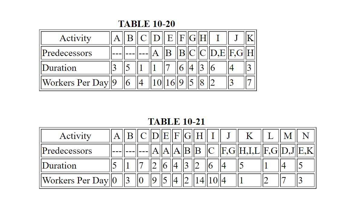
(11 to 12) For the projects described in Tables 10-20 and 10-21, respectively, suggest a project schedule that would complete the project in minimal time and result in relatively constant or level requirements for labor over the course of the project. Compare the minimum duration of the project with no resource constraints and the duration that results from your suggested schedule. Use your own choice of scheduling software unless otherwise directed by a course instructor.
(13) Develop an example of a project network with three critical paths.
(14) For the project defined in Table 10-20, suppose that you are limited to a maximum of 20 workers at any given time. Determine a desirable schedule for the project, using the late start time heuristic described in Section 10.9.
(15) For the project defined in Table 10-21, suppose that you are limited to a maximum of 15 workers at any given time. Determine a desirable schedule for the project, using the late start time heuristic described in Section 10.9.
(16) The examples and problems presented in this chapter generally make use of activity duration and project durations as measured in working days from the beginning of the project. Outline the procedures by which time measured in working days would be converted into calendar days with single- or double-shift work. Could your procedure be modified to allow some but not all activities to be underway on weekends?
10.12 Footnotes
- See Au, T., Introduction to Systems Engineering, Deterministic Models, Addison-Wesley Publishing Company, Reading, MA, 1973, for a detailed description of linear programming as a form of mathematical optimization.
- See K.C. Crandall, “Project Planning with Precedence Lead/Lag Factors,” Project Management Quarterly, Vol. 4, No. 3, Sept. 1973, pp. 18-27, or J.J. Moder, C.R. Phillips, and E.W. Davis, Project Management with CPM, PERT and Precedence Diagramming, New York: Van Nostrand Reinhold Company, third edition, 1983, chapter 4.
- See C.T. Hendrickson and B.N. Janson, “A Common Network Formulation of Several Civil Engineering Problems,” Civil Engineering Systems, Vol. 1, No. 4, 1984, pp. 195-203.
- See IBM, Project Management System, Application Description Manual, (H20-0210), IBM, 1968.
- A variety of mathematical programming techniques have been proposed for this problem. For a review and comparison, see J.H. Patterson, “A Comparison of Exact Approaches for Solving the Multiple Constrained Resource Project Scheduling Problem,” Management Science, Vol. 30, No. 7, 1984, pp. 854-867.
- This example is adapted from H. Smallowitz, “Construction by Computer,” Civil Engineering, June, 1986, pp. 71-73.
- For discussions and comparisons of alternative heuristic algorithms, see E.M. Davies, “An experimental investigation of resource allocation in multiactivity projects,” Operational Research QuarterlyVol. 24, No. 11, July 1976, pp. 1186-1194; J.D. Wiest and F.K. Levy, A Management Guide to PERT/CPM, Prentice-Hall, New Jersey, 1977; or S.R. Lawrence, A Computational Comparison of Heuristic Scheduling Techniques, Technical Report, Graduate School of Industrial Administration, Carnegie-Mellon University, 1985.
