EXPERIMENT 10: FLUID FLOW
Introduction
Liquids only flow through pipes if forced to do so by pressure caused by a pump of by gravity. It is found that the pressure measured at any point in the pipe decreases in the direction of flow. This pressure loss is caused by friction in the liquid and between the liquid and the walls of the pipe.
The fluid flow apparatus in room E030, shown in Figure 1 consists of a small pump pumping water from a holding tank through a series of pipes and back into the tank, to form a closed loop. The piping contains a number of valves that can be used to force the water to flow through any or all of the five sections shown, depending on which valves are open or closed. If all the valves are closed no water will flow. This would damage some pumps but not the centrifugal pump used in the lab.
The piping system also contains a rotameter (flowmeter), a line with an orifice plate, a line with a venturi, a line with round and square bends, and line with an expansion / contraction section, and a line with a globe valve and a gate valve. Along the pipes are many pressure tappings where pressure can be measured. This is done via pressure transmitters which report the pressure in inches of H2O.
For fluids flowing in a piping system where the pipes are full, the pressure change from one position to another can be calculated from Bernoulli’s formula which, assuming there is no pump between points 1 and 2, yields:
(1) 
where:
- z1, z2: heights of water in the piping system relative to a common reference height (m)
- V1, V2: velocity of water (m/s)
- P1, P2: static pressure in the pipe (Pa = kg/(m s2))
- ρ: density of water (kg/m3)
- g: gravitational acceleration (9.81 m/s2)
- hL “head loss” which accounts for energy loss due to friction (m)
When the diameter of the pipe does not change, the velocity will also remain constant and Bernoull’s equation reduces to:
(2) 
When there is also no change in elevation (e.g. the piping is horizontal), the height terms can also be eliminated and Bernoulli’s is simplified to:
(3) 
Thus, any change in static pressure is due only to friction loss.
In the case of the Venturi tube and the orifice plate, where there is a dramatic decrease in pipe diameter there is also a change in the fluid velocity. This is because the same flow of water must be pushed through a changing pipe diameter and this can only happen with a change in velocity. The volumetric flow rate of water through a pipe is given by:
(4) 
where Q is the volumetric flow rate in m3/s and A1 is the cross sectional area of the pipe in m2.
As the flow, Q, cannot change (mass conservation requires that Q1 = Q2 for an incompressible liquid), when the cross sectional area decreases, (A1 > A2), the velocity must increase correspondingly (V2 > V1). Through Bernoulli’s equation, this dramatic increase in velocity results in a sudden pressure drop. Another way to look at this is that Bernoulli is an energy conservation equation. As the fluid goes through a constriction in the flow it picks-up speed and kinetic energy. This kinetic energy must come at the expense of another type of energy of the fluid which in this case is pressure. Hence, at the “throat” of the Venturi tube the speed increases and the pressure decreases. This drop in pressure can be used to calculate the flow through the pipe, which is what Venturi tubes are used for:
(5) 
Where
- Q is the volumetric flow rate (m3/s)
- C is the discharge coefficient, typically 0.98 –1.02
- A1 is the cross sectional area of the pipe before the constriction (m2)
- A2 is the cross sectional area of the throat (narrowing) (m2)
- g is the acceleration due to gravity (9.81 m/s2)
- H1, H2 are the pressures right before the Venturi (H1) and at the throat (H2) (both in meters of H2O)
The fluid flow system in room E030 consists of a tank, a pump, and five lines in parallel. A photo of the equipment with several key elements is provided below.
Figure 1: Fluid Flow apparatus in E030
The apparatus has been automated and most of the functions are controlled through an operator station. A screenshot of the operator station with key elements is provided below
Figure 2: Operator station for Fluid Flow apparatus in E030
Purpose
The purpose of the experiment is:
- To calibrate the rotameter (to find the equation of the line relating rotameter reading to actual mass flow rate)
- To find the pressure profile along the orifice section of the apparatus and examine how it depends on flow rate
- To find the pressure profiles along the venturi section of the apparatus and examine how it depends on flow rate
- To investigate the relationship between pressure drop and flow rate.
- To determine the volumetric fluid flow based on the pressure drop through the Venturi and compare that value to the rotameter reading.
Procedure
Before proceeding, check your understanding of key elements of the apparatus by performing the following drag-and-drop task.
Drag the text descriptions to the corresponding place on the image of the Fluid-Flow Apparatus
Part I: Calibration and Pressure Profile
Only the top two sections (Orifice & Venturi) are used in this part. The calibration of the rotameter can be done simultaneously with measurement of the pressure readings. The calibration can be done on either the venturi or orifice line; however, both lines will be run for the pressure profile.
- Preparation:
- Make sure the water level in the tank is at least 2/3 full; otherwise air can be drawn into the pump. If the level is low, use the hose on the side (next to the safety shower) to fill the tank.
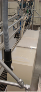
Figure 1: Tank of fluid-flow experiment - Open the rotameter valve then the inlet and outlet valves of the first line. Make sure all other valves are closed. With the switch behind the rotameter (see figure below), turn on the pump.
- Set the flow of water to 700 (look at the picture below to see how to properly read the flow of water) to allow all the air bubbles stuck inside the pipes to escape. This might take some time… let the water run for a bit.
- Make sure the water level in the tank is at least 2/3 full; otherwise air can be drawn into the pump. If the level is low, use the hose on the side (next to the safety shower) to fill the tank.
- Measurements on first line:
For the first line, you will be doing two tasks simultaneously: record the pressure on the line and check the rotameter flow rate at different rotameter settings- Set a flow of water of 100 IGPH (imperial gallons per hour) by adjusting the rotameter valve. Make sure there are no air pockets in the line (if there are any, go back to step 3 of the preparation). Record the flow rate shown by the rotameter float (read from the centre shoulder of the float). Write down the units of the rotameter.
- Check (calibrate) this flow rate by diverting the water going back to the tank into a weighed bucket and measuring the mass of water collected over a measured period of time (use 30 seconds or 60 seconds). After your measurement return that water to the tank.
- At the operator’s station, be sure that the appropriate line (venturi or orifice) is selected. Record the pressures at each of the tappings as displayed on the operator’s screen and transducers. Wait about 30 seconds after adjusting the flow rate before recording the pressure values. The values will still be oscillating; take an average value if possible. Recall that the units of pressure are inches of water column (“H2O).
- Repeat seven times, for a total of 8 different flow rates, using different flow rates by adjusting the rotameter valve. Try to obtain eight sets of readings which cover the whole range of rotameter flows as shown by the scale.
- If any result is suspect, repeat the measurement.
- Measurements on second line:
- Close the valves for the first line and open those for the second line. Follow the procedure shown in the video to avoid over-pressurizing any line.
- At the operator’s station, be sure that the Venturi (second) line is selected.
- Turn the rotameter valve to set the flow rate to its maximum. Let the water run for some time to allow all the air bubbles stuck inside the pipes to escape.
- Repeat the pressure recording procedure (steps 3, 4, and 5 from first line above) for the second line (venturi), but this time only the pressure profile information needs to be collected. Make sure you collect pressure readings over at least eight flow rates that span the whole range of rotameter values.
- Stop Down
- At the end of the experiment, stop the pump. Turn the rotameter to zero and open all of the valves for the top line.
- At the operator’s station, select the “none” button.
Report
Part I
Present all your data through Tables. Make sure your table contain proper units
- Calibration curve
- Use your “calibraton data” (i.e. the actual flow rate data collected by diverting the water into a bucket and weighing) to calculate the actual flow rate through the pump in kg/s.
- Create a plot of actual flow rate vs. Rotameter reading.
- Find the equation of the line graph. It must cross the origin. This equation will be used for converting all rotameter readings to actual flow rate
- Comment on the accuracy of the rotameter reading. You can do that by comparing the rotameter reading (convert from IGPH) to the actual flow rate. Check below if your conversion is correct:
- Pressure profiles for orifice section
- For each flow rate, plot the pressure value on the y-axis versus the pressure point number on the x-axis. Place the data from all flowrates on one graph. Label the axes and provide a clear graph legend.
- Comment on the graph. How does the orifice affect the pressure through the line? How does the pressure profile change as the flow rate increases? Are there any anomalies in the data points?
- Pressure profiles for venturi section
- For each flow rate, plot the pressure value on the y-axis versus the pressure point number on the x-axis. Place the data from all flowrates on one graph. Label the axes with units, if needed, and provide a clear graph legend.
- Comment on the graph. How does the venturi affect the pressure through the line? How does the pressure profile change as the flow rate increases? Are there any anomalies in the data points?
- Compare the venturi line pressure profile to that of the orifice line. Was the maximum flow rate the same for both lines? If not, why?
- Pressure drop vs flow rate
- For the orifice line, calculate the overal pressure drop through the line at each flow rate. The overall pressure drop is the pressure at the first tapping minus the pressure at the last tapping (P1 – P6).
- Plot the overall pressure drop on the y-axis versus the flow rate on the x-axis. Use logarithmic scales for both axes.
- Comment on the shape of the graph and any scatter of the data points. How does the flow rate affect the pressure drop?
Part II
Present all your data through Tables. Make sure your tables contain proper units. Use the data from the venturi (second line) for this part of the report.
- For each flow rate, use equation 5 in the introduction part to calculate the volumetric flow rate based on the pressure differential through the Venturi. Note the following:
- Assume a discharge coefficient of 1.00
- Use the pressure value right before the throat and at the throat of the venturi tube (you do not need all pressure measurements)
- Convert the pressure values to meters of water column (simply convert the inches of water to meters of water)
- The diameter of the throat is given at the end of the manual.
- For each flow rate convert the rotameter reading to actual flow rate. Use the calibration curve derived in Part I. That curve provides mass flow rate in kg/s; convert that to volume flow rate using the density of water (1000 kg/m3)
- Compare the flow rate value calculated through the venturi pressure drop (step one above) to that calculated through the calibration curve (step 2 above). For each flow rate setting, calculate the coefficient of discharge (i.e. the correction factor) of the venturi:
(6)

Calculate the average coefficient of discharge by averaging the coefficient values calculated for the flow rates you have readings for.
Useful dimensions
- Orifice:
- pipe diameter: 39.9 mm
- throat diameter: 22.2 mm
- Venturi:
- pipe diameter: 38.8 mm
- throat diameter: 14.6 mm