Introduction

All material, including Figures is taken from CE583-ADSORPTION, 2014, G.U.N.T, Gerätebaum, Barsbüttel, Germany, unless otherwise noted.

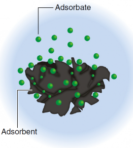
Adsorption refers to the attachment of substances from a liquid or gaseous phase to solids. The solid is referred to as the adsorbent. The substance taken up is called the adsorbate.

In adsorption there is a fundamental difference between Physisorption and Chemisorption. In physisorption the attachment of the adsorbate is based on physical forces (Van der Waals forces). In contrast, during chemisorption the adsorbate enters into a chemical bond with the molecules of the adsorbent. In physisorption there are significantly lower binding energies than in chemisorption. Therefore, adsorption processes based on physisorption can usually be reversed. This makes desorption of already adsorbed substances possible.

The term loading of an adsorbent means the mass of adsorbate that has been adsorbed by one gram of adsorbent. The loading is therefore stated in units of mg/g.

Activated carbon

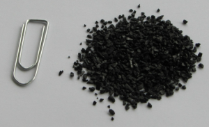
In water treatment it is almost always activated carbon that is used as the adsorbent. Therefore, the following explanations are restricted to activated carbon. In the case of activated carbon, the adsorption processes are mainly based on physisorption. The largest part of activated carbon is microcrystalline carbon, but around one third consists of amorphous carbon and mineral content (ash). Source materials for producing activated carbon include carbon-containing raw materials such as: Black coal, Brown coal (lignite), Charcoal, and Coconut shells.

The most commonly used production process is activation with water vapour. This process consists of using water vapour to heat the source material to temperatures of approximately 800 to 1000°C. This causes the vast majority of the carbon to turn into gas. As a result of this gasification, a widely branched pore system develops in the carbon particles. This is where activated carbon gets its high adsorption capacity in comparison to other adsorbents.

The surface of activated carbon is usually hydrophobic. Therefore, activated carbon is particularly suited to the adsorption of polar, organic substances. Activated carbon has an extensively branched pore system, which is one of its key properties. The pore diameter in this system is in the scale of approx 0.4 to 100nm.  Pores are categorized depending on their size:

• Micropores: 0.4 to 1 nm
• Mesopores: 1.0 to 25 nm
• Macropores: 25 to 100 nm

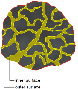
When talking about the activated carbon surfaces we have to differentiate between the inner and outer surfaces.

• Outer surface: The outer surface of an activated carbon particle is crucial for the mass transfer on the surface of the particle.
• Inner surface: The inner surface of an activated carbon particle is equal to the overall surface of all pores. The actual adsorption of the adsorbate takes place on the inner surface, which makes up more than 95% of the total surface area of an activated carbon particle.

Adsorption is defined by the structure and size of the pores. Therefore, the pore surface is a very important parameter for characterising activated carbon. The pore surface of one gram of activated carbon is in the scale of 1000 m². In other words: 5 grams of activated carbon have roughly the same pore surface area as a football field!

Dynamics of Adsorption

In the field of water treatment, adsorption is usually carried out with adsorbers that are in continuous operation.  In these, water continuously flows, from top to bottom, through an immobilized layer (often called a “fixed bed”) of granulated activated carbon. This set-up can also be used for other process, as for example dehydration of natural gas as shown in Figure 4.

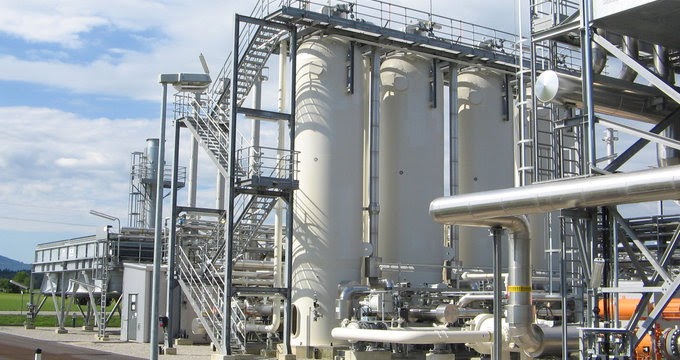
Figure 4: Natural gas dehydration plant – Silica Verfahrenstechnik GmbH, Visual Encyclopedia of Chemical Engineering: Adsorption (n.d.), http://encyclopedia.che.engin.umich.edu/Pages/SeparationsChemical/Adsorbers/Adsorbers.html

In this fixed-bed set-up, the loading stage of the adsorbent must be closely monitored, because as adsorbate continuously passes through the column, the adsorbent slowly becomes saturated.  Recall that the adsorbate gets physically attached to the porous surface of the activated carbongets slowly .  The available surface becomes gradually fully covered  and the activated carbon becomes saturated.  It then needs to be removed from the process and re-activated.

Activated carbon can then assume the following three states in an adsorber:

• State 1: The activated carbon is completely loaded and can therefore not take in any more adsorbate.
• State 2: The activated carbon is partially loaded and can therefore still take in more adsorbate.
• State 3: The activated carbon is completely unladen and still has its original capacity.

The determination of the state of the activated carbon (or any adsorbent) is done by monitoring the concentration of the adsorbate through the column.  A typical concentration profile is show in Figure 5, where the three stages mentioned above are noted.  At the top of the column the adsorbent is completely loaded, further down it is partially loaded, and towards the bottom it is unladen (contains no adsorbate).

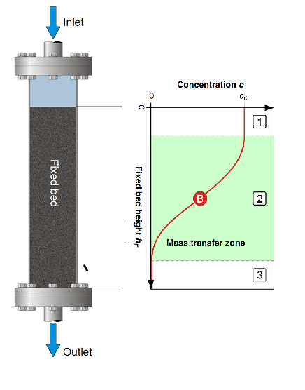
Figure 5: Typical adsorbate concentration profile through a fixed-bed adsorption column

Over time, as more water and adsorbate pass through the column, more of the adsorbent becomes loaded and the concentration profile changes as shown in Figure 6.  At time t₁ there is no adsorbate leaving the column (all gets adsorbed in the adsorbent).  However, at time t₂ there is some adsorbent leaving the column with a concentration C₂, which increases to C₃ at time t₃.

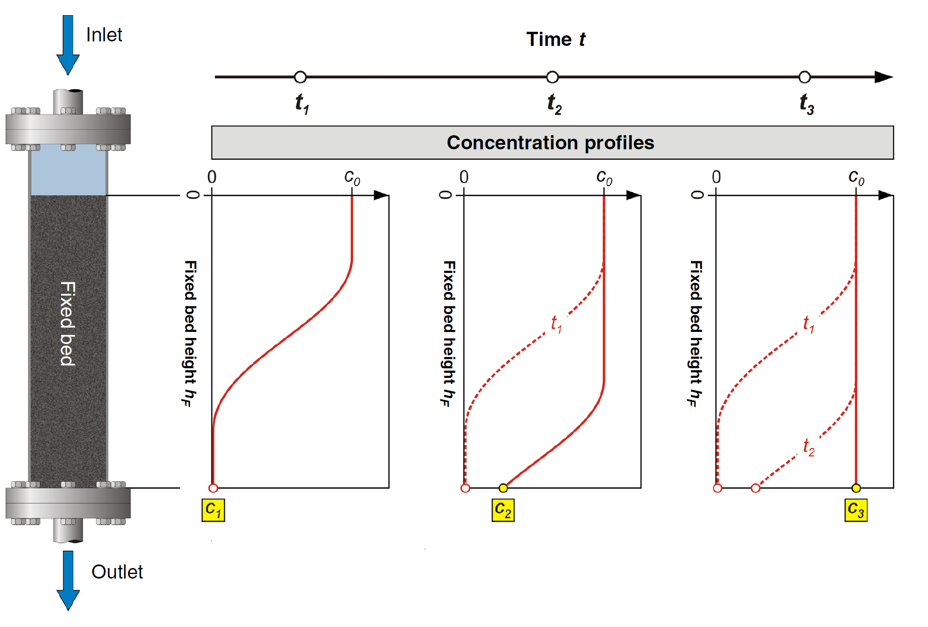
Figure 6: Change of adsorbate concentration through fixed-bed column over time of operation.

This outlet adsorbate concentration is extremely important in the operation of an adsorption process, as it often has a maximum allowable value imposed by process requirements or environmental regulations (recall that adsorption is usually performed to remove a contaminant from a liquid or gas stream).  The evolution of this outlet concentration over time is called the breakthrough curve of the column.  It can be generated by collecting the data (C₁, C₂, and C₃) from the curves in Figure 6.  Alternatively, it is customary to rotate the concentration profiles of Figure 6 by 90 degree counter-clockwise, plot them all in one graph and then use the outlet concentration to develop the breakthrough curve, as shown in Figure 7.

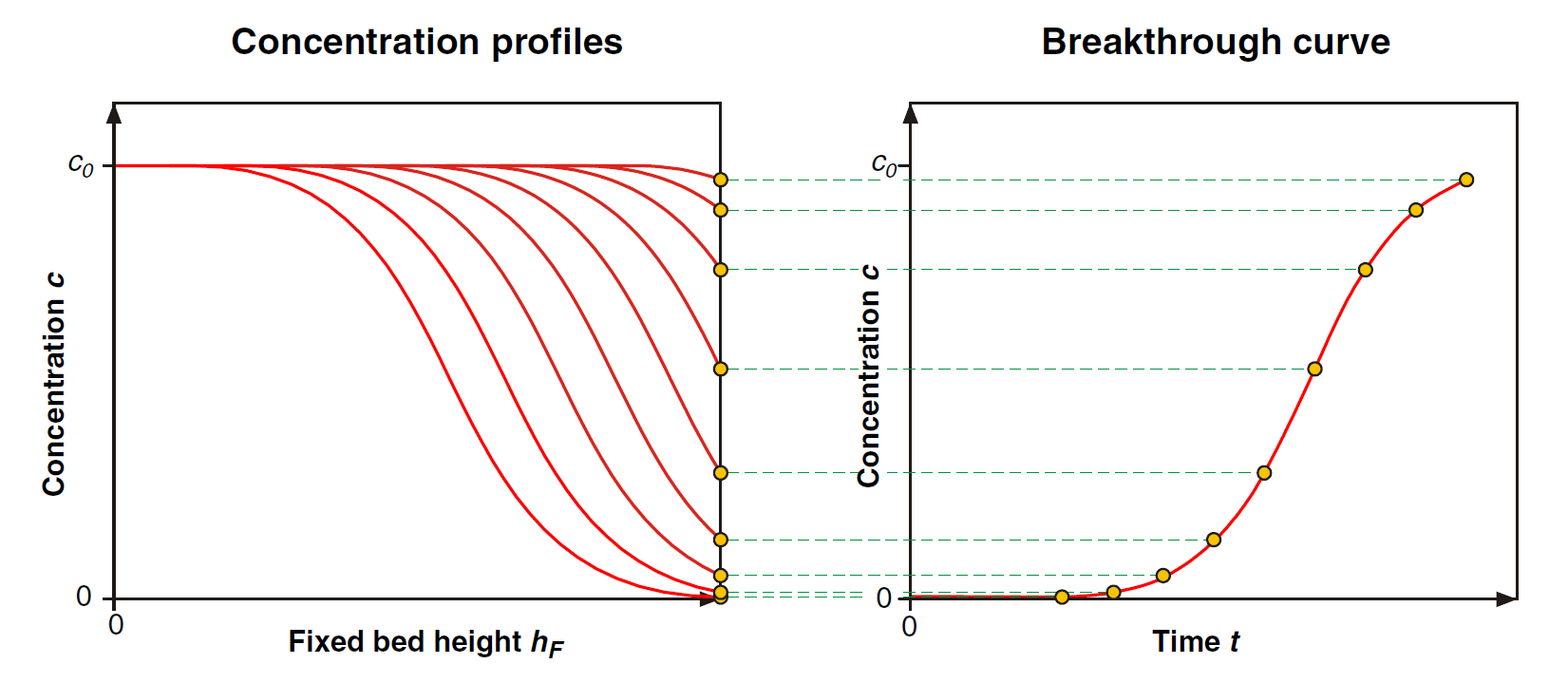
Figure 7: Creation of a column breakthrough curve from time evolution of the adsorbate concentration profile.

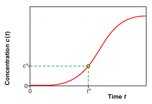
From a brakthrough curve, the time of breakthrough can be calculated.  The time of breakthrough is the time t^* when the outlet concentration of the adsorbate reaches the acceptable maximum concentration C^*, as shown on Figure 8.  Once that point is reached, the adsorption on this column must be stopped and the adsorbent regenerated, if possible, or replaced.

In continuous operations, taking the adsorption unit off line to regenerate the adsorbent is not practical, as it requires stopping the process.  To overcome this, multi step units are used where several adsorption units are arranged in series, as shown in Figure 9.

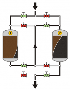
The advantage of such a set-up is that once the left-hand-side (first in line)unit is loaded with adsorbate, it can be replaced while the process relies momentarily only on the second adsorbent.  Once the left-hand-side column is replaced, the valves on top can be changed to place it second in the series (liquid will go first through the right-hand-side column and then through the left-hand-side one).  That way, the right-hand-side unit will became loaded next at which point it will be replaced and so on.

You can test your understanding of this introduction to adsorption by trying the summary questions below.  Pick the correct statement from each set of statements.

Adsorption Unit

The adsorption unit in E030 is the CE 583 from G.U.N.T, Gerätebau GmbH.  The main components of the unit are two adsorption columns placed in series.  Multiple taps are added to the first column to take samples for concentration measurements.  A photo of the equipment with major components outlined is given in Figure 10.

Figure 10: Adsorption column in E030 with features highlighted.

A schematic of the whole unit is provided in Figure 11.  The unit contains two reservoirs, one “concentrated water” tank (B2) with fresh water to be cleaned and one “Treated water” tank (B1) with water that has already gone through the columns. Both tanks are equipped with pumps to push liquid from either tank, or a mix of both, through the adsorption columns.  The flow through the system is adjusted through a regulating valve (V15) and measured by a flow meter (FI).  A heater with a control loop is installed on the treated water tank to heat-up, if needed, liquid that will be recirculated through the columns.

Figure 11: Schematic of adsorption column unit

During normal operation, the pump P1 pumps the fresh water from tank B1 to the first adsorber (A1). A concentrated adsorbate solution is dispensed into the feed line to the adsorber by the concentrate pump P2. Mixing the fresh water (1) with the concentrated adsorbate solution (2) results in the raw water (3), as shown in Figure 12 The concentration of the adsorbate in the raw water depends on the mixing ratio of the two flow rates. The mixing ratio can be adjusted via the flow rates of the two pumps.  The adsorbate adsorbs on the activated carbon in adsorber A1 and is thus removed from the raw water. The treated water goes down back out of the adsorber and then flows through the second adsorber (A2), which is also filled with activated carbon. The water that comes out of the second adsorber is discharged back into tank B1 and is pumped back into adsorber A1 once more. In this way there is a closed water circuit for the treated water. Adsorber 2 therefore functions as a safety adsorber. This ensures that the water doesn’t contain any more adsorbate, including when it breaks through the first adsorber.

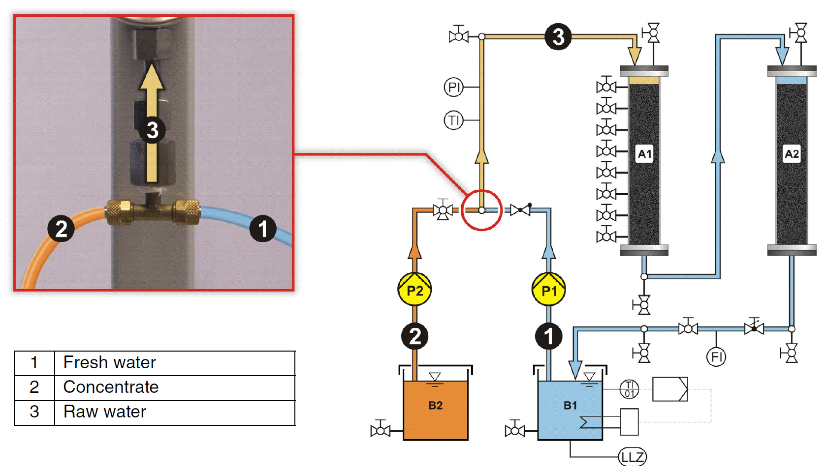
Figure 12: Explanation of the mixing process of fresh water and concentrate to give raw water fed to the adsorbers.

You may check your understanding/knowledge of the unit by trying the “Drag-and-drop” exercise below.  Drag the descriptions on the left to the location of the item on the unit photo.

Purpose

The purpose of this experiment is to determine the effectiveness of activated carbon for the removal of methylene blue dye from water and to create concentration profiles for an adsorption column.

Procedure

Fixed Bed Height Determination

To determine the fixed bed height h_F,max, measure the distance, h_F^*, between the top sampling valve V5 and the top edge of the bed of activated carbon. The value should be in the range of 2 to 5 cm. The overall height of the fixed bed h_F,max is: h_F,max = (h_F^* + 41.5) in cm. Determine the depth, in cm, for each sampling tap V5 to V13, knowing h_F^* (enter values in data tables below). The sample from V16 will be representative of the concentration at the top of the filter bed h_F = 0.0 cm. Note: Sample valve V14 is located at the bottom of the second column.

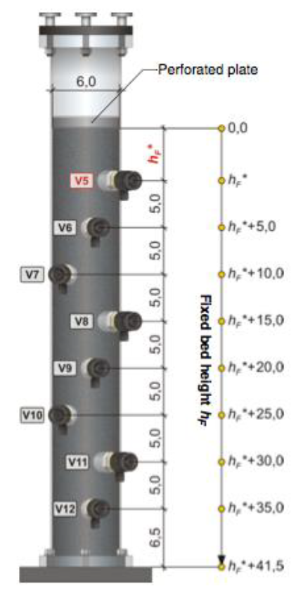
Figure 13: Location of sampling taps on 1st adsorption column.  All distanceσ in cm.

Experimental Procedure

1. Clean 20 screw cap sample tubes with methanol and rinse with distilled water to remove any staining. Caps are not needed for the tubes.
2. Check that a hose is connected to the over- flow outlet on the treated water tank B1. The other end of the hose must be located in a drain in the floor.
   

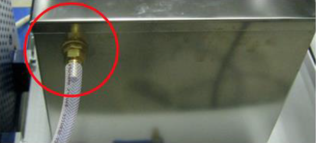
   Figure 14: Tank overflow outlet

    

3. Open the regulating valve V15 by turning the knob counter-clockwise as far as it will go.
   

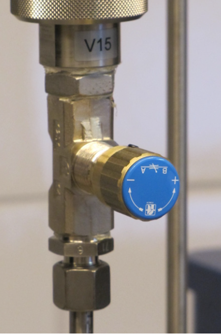
   Figure 15: Regulating valve V15

4. Bring the valve V3 into the position shown below to open valve V3.
   

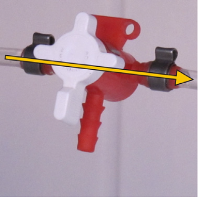
   Figure 16: Three-way valve V3

    

5. Check that all other valves are closed.
6. Completely fill the treated water tank B1 with tap water.
7. Ensure that the suction line to the concentrate pump P2 is in the bottle of concentrated methylene blue solution (Tank 1).
8. Start the circulation pump on the main panel.
9. Use the potentiometer to adjust the speed  of pump P1 so that it is pumping at 25 L/min.  The flow rate is read from the flow meter F1.
   

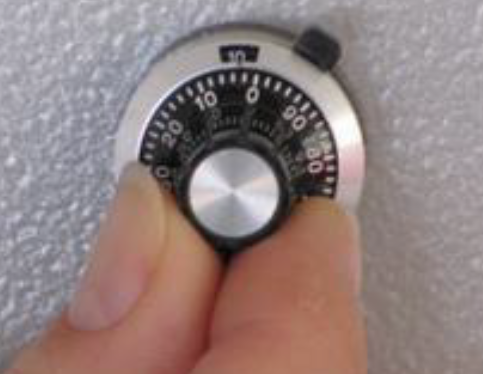
   Figure 17: Flow-adjusting potentiometer.

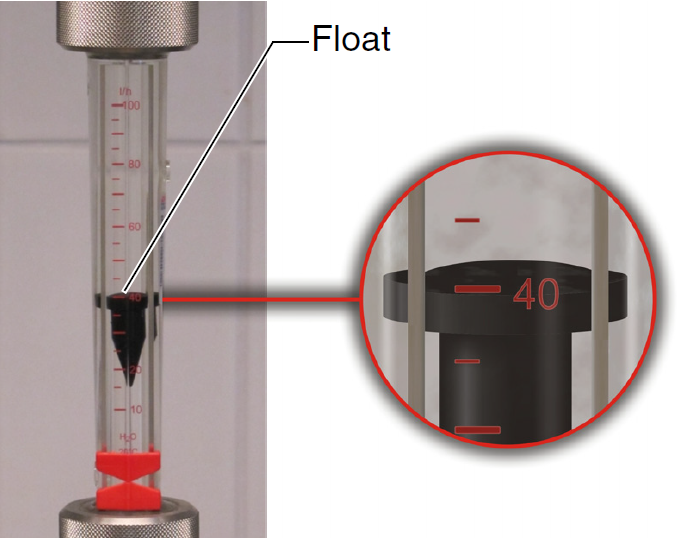
   Figure 18: Flowmeter.  Measure flow rate at the top of the float

10. Leave the heater off for this experiment.
11. Turn the concentrate pump P2 on by pressing the start/stop button (Figure B in Figure 19, below).
    

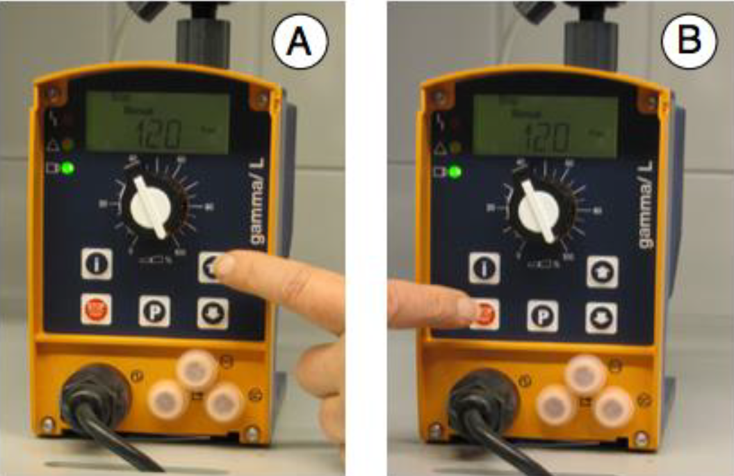
    Figure 19: Concentrate pump.  A. Frequency adjustment. B. Start/Stop button.

12. Press the information button (i) to switch between stroke length and frequency.
13. Set a relative stroke length (SL) on the pump P2 of 50%. (Figure Aof Figure 19, above)
14. Set the frequency (f) on pump P2 to 75 min^-1.
15. Start a timer.
16. After about 15-minutes take samples from V16 and V5 to V14 in the test tubes provided. Open each valve (one-at-a-time) and allow sample to flow for a few seconds into a beaker before collecting the sample in the tube.
    

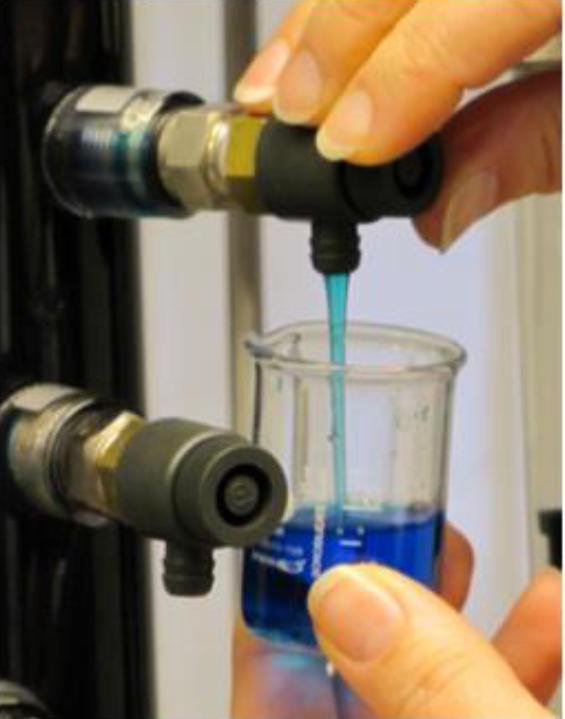
    Figure 20: Sample collection

17. Measure the absorbance of the samples using the Hach DR3900 spectrophotometer with a wavelength of 610 nm. Distilled water should be used as a reference blank.
18. Also, measure the absorbance of a set of reference samples with methylene blue concentrations between zero and 10 ppm.
19. Collect and measure the absorbance of a second set of samples from each valve (V16 and V5 to V14) after at least 60 minutes have elapsed from the beginning of the experiment. Note down the time of sample collection.
20. Stop the experiment by stopping both pumps.
21. Flush the line from the concentrated methylene blue solution with distilled water.
22. Drain the treated water tank B1 and remove any remaining liquid in tank B1 using the provided sponge.

Report

A sample Table for most measurements and calculations is provided at the end of this section in Figure 22.  Please, refer to it, if needed

1. Create Tables with all your measurements:
   • Absorbance from all sampling taps at time of 15 minutes and 60 minutes
   • Absorbance from all standard solutions.
   • Fixed-bed height of all sampling taps.
2. Use the absorbance values of your standard solutions to create an absorbance / concentration plot.  Your plot must have proper axes labels with units.  Run a trendline (best-fit line) through your data, making sure, through, that your trendline crosses through the origin (0,0), as zero absorbance corresponds to zero concentration.
3. Use the trendline equation to convert your absorbance readings to concentrations. Report in a Table and do not forget to include units on the column or row titles.
4. Normalize concentrations by dividing by the initial concentration at the top of the column (V16).  After normalization, all “concentrations” must be in the range of zero to one.  Tabulate your results.
5. Create concentration profiles for the column by plotting Normalized concentration (y-axis) versus fixed bed height (x-axis). Plot both profiles for 15 minutes and 60 minutes on one graph. (see sample graph below)
   

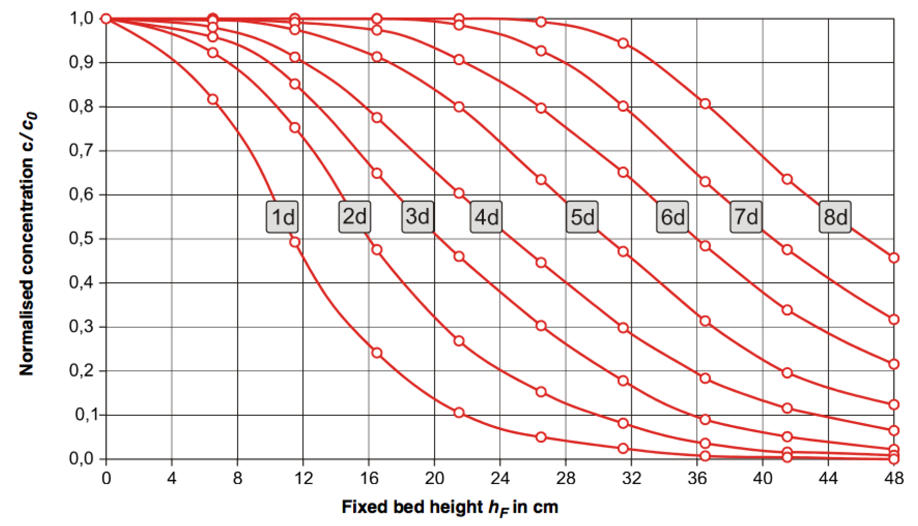
   Figure 21: Normalized concentration profile in adsorption column.  Concentration profiles after continuous operation for one to eight days are shown.

6. Discuss the shape of the concentration profile. Does it make sense? Explain your reasoning?
7. Describe sources of error for the experiment.
8. Describe an application where activated carbon treatment might be used.

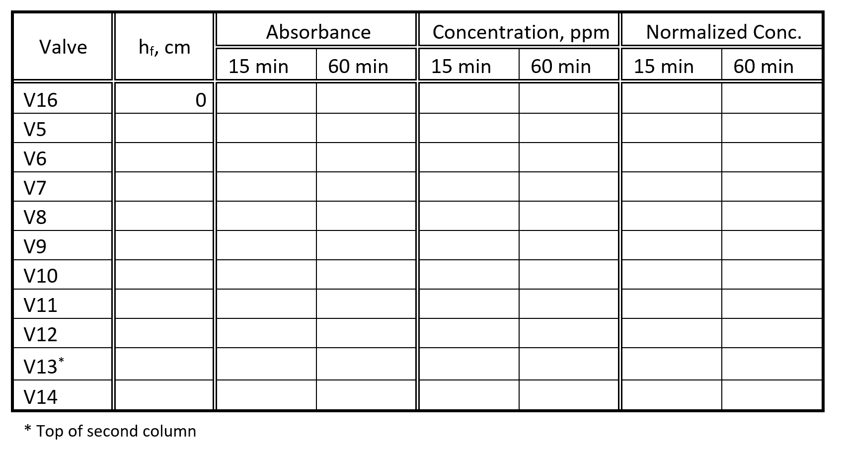
Figure 22: Sample Table for absorbance measurements and calculations