Machine Learning in The Digital Humanities
INTRODUCTION
Machine learning (ML) is a subfield of computer science and mathematics that studies algorithms that improve their performance, or “learn” with experience and utilization of data. What is meant by “experience”, “learn” and “data” requires clarification and development. However, some alternative definitions provide context for the discussion.
In a web article for the MIT Sloan School of Management, Sara Brown writes: “Machine learning is a subfield of artificial intelligence, which is broadly defined as the capability of a machine to imitate intelligent human behavior. Artificial intelligence systems are used to perform complex tasks in a way that is similar to how humans solve problems.”
Karen Hao, Senior AI Editor for the MIT Technology Review, provides another definition: “Machine-learning algorithms use statistics to find patterns in massive amounts of data. And data, here, encompasses a lot of things—numbers, words, images, clicks, what have you. If it can be digitally stored, it can be fed into a machine-learning algorithm.” She summarizes machine learning as follows: “Machine-learning algorithms find and apply patterns in data. And they pretty much run the world”
In the web journal Towards Data Science, machine learning engineer Gavin Edwards provides a definition that underscores the importance of data in machine learning: “Machine learning is a tool for turning information into knowledge. In the past 50 years, there has been an explosion of data. This mass of data is useless unless we analyse it and find the patterns hidden within. Machine learning techniques are used to automatically find the valuable underlying patterns within complex data that we would otherwise struggle to discover. The hidden patterns and knowledge about a problem can be used to predict future events and perform all kinds of complex decision making.”
Machine learning has a connection to artificial intelligence and constitutes a very large area of study. For the purposes of motivating an investigation of machine learning in the context of the digital humanities, it suffices to note that machine learning algorithms are adaptive algorithms that improve their performance through the data on which they act in combination with specialized optimization (“learning”) approaches. Optimization is the basic paradigm of many machine learning algorithms. Machine learning algorithms use sample data, called training data, as their input to generate a mathematical model for prediction, classification, or decision making. The resulting model is not programmed to make these predictions, classifications, or decisions. These capabilities emerge from the model based only on the training data.
There are several classes, or models, of machine learning algorithms. The term “model”, used in this way, is not to be confused with the prediction models described above. Machine learning algorithms produce useful models to study and analyze various phenomena, but in the discussion below, the term “model” refers to a broad class of machine learning algorithms. Following the literature on machine learning, “models” will have both meanings in the following discussion, which will be clear from the context.
Supervised Learning
In supervised learning models, training data are labeled. Given a d-dimensional point, or vector (a datum consisting of d values) with a label, supervised learning attempts to construct a mapping between that d-dimensional data point and its label. In this way, supervised learning is “learning by example”. With a large number of varied examples, the training of the model is better, and consequently, the learning is better. Generally, a greater number of labeled examples results in a better mapping, and a higher performance of the model. A canonical example of supervised learning is handwriting recognition, in which handwritten alphanumeric characters are input into a supervised model, and the model reports which character was input. Recognizing objects in images is another application of supervised machine learning. This learning method is supervised because the labels are assigned by humans, and humans select the training data. The entire process is “overseen” by human users.
For supervised learning models to be useful, they must generalize what they “learn” based on the examples provided. For instance, in the handwriting recognition example, if 300 examples of a handwritten digit “7” characters are input by 300 different writers, a model that was successfully trained would recognize the digit 7 written by a different, 301th writer. The model “learned” a mapping from its examples and can label new input on which it was not trained. Generalization is the adaptation of the model to new examples, based on the examples on which it was trained. There are, however, difficulties that must be avoided, or at least reduced, in supervised training. One such problem is overfitting, where the model “memorizes” its input. Overfitting is often manifested with very high training performance with low error, but the model does not generalize when presented with new input. Another issue inherent in supervised training is the problem of bias. The model can only “learn” from the input examples it is provided, and therefore a sufficiently representative set of training data must be provided. Bias underscores another aspect of the human-in-the-loop aspect of supervised machine learning – that training examples must be chosen carefully. The human user must therefore provide reliable, or correctly labeled, unbiased samples.
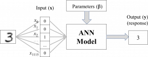
Artificial neural networks (ANNs) are prototypical examples of supervised machine learning models. For instance, using the example above, an ANN model can be “trained” to recognize handwritten digits 0, 1, …, 9, using many images of handwritten digits and their associated “true” labels (e.g., an image of a handwritten “3” would have a label of 3) as the training data. The images themselves are represented as pixels (picture elements) and can be represented in a list of values. For example, an image of size 31 x 36 (31 rows and 36 columns) can be “flattened” to 1,116 (= 31 x 36) binary values containing 0s and 1s, where 0 (black) indicates a pixel that is part of a digit, and 1 (white) indicates a pixel that is part of the background (or conversely). This model can be represented graphically, as shown below.
Artificial neural networks will be discussed in detail in a later section.
Supervised learning Applications
Classification is assigning each input vector, or d-dimensional input point, to a class. For instance, a supervised learning model may be trained to classify images of dogs, moose, and cats, into the classes: “dog”, “moose”, and “cat”. Presented with a new, “unseen” image of a moose on which the model was not trained, the model, if trained properly, will return “moose”. In other words, the output of the supervised learning model is a discrete class.
Regression
In regression, given an input vector, the output of the machine learning model is a number, or vector of numbers, instead of a discrete class. For instance, consider a simple model, the equation of a line: y = mx + b, where x is an independent variable, m is the slope of the line, and b is the y-intercept. Given a large number of (x, m, b) training vectors labeled with the output y as training data, the supervised model will be able to “compute” y = mx + b when new (x, m, b) vectors are presented, although the model was not trained on this vector. In other words, the model formulates a mapping that solves the equation y = mx + b, by returning y as its output.
Unsupervised Learning
Unsupervised learning also uses data for self-adaptation. However, unlike supervised learning, the data are not labeled. The purpose of unsupervised learning is for the machine learning algorithm to discover patterns, anomalies, and/or other interesting features in the input data, based only on those data, without a human user pre-specifying those patterns, anomalies, or features. In most cases, the user does not have a well-formed idea of what may be found in the data for a variety of reasons. The data may be excessively large, heterogeneous, or complex, for example, and, as a result, machine learning is employed to uncover what may not be evident or obvious to users. Unsupervised learning is therefore used for knowledge discovery (Gavin, Introduction).
One of the main applications of unsupervised learning is clustering. In clustering, data are placed into groups, categories, or clusters, based on some feature inherent in the data themselves. Clustering algorithms therefore find an optimal separation between clusters of data, based on some optimality measure. However, in many clustering algorithms, human users usually decide the number of clusters, and consequently, these algorithms cannot be said to be completely without human intervention. The most widely used and relatively simple clustering approach is the k-means algorithm. In this method, the user specifies the desired number of clusters, denoted as k (hence the name “k-means”). This iterative method starts by assigning data samples of any dimensionality to a cluster label, usually integers from 0 to k – 1. The centroid, or mean, of the data for each dimension of each of the k clusters is calculated. In the following step, some distance measure between each data sample and the centroids of each of the k clusters is determined. The Euclidean distance (the standard distance calculated from the Pythagorean Theorem; more details are presented in a subsequent section) is usually employed. Each data sample is then re-assigned to the cluster to which it is closest. The re-assignment changes the centroids of the clusters, as the original centroids were computed based on the original assignment, not the new one resulting from re-assignment. Therefore, the centroids of the k clusters must be re-calculated. In the next step of the algorithm, the centroids are re-computed, followed by re-computing the distances from each data sample to the (new) cluster centroids. Data samples are then re-assigned based on these distances. Therefore, the basic algorithm consists of
- computing the k cluster centres;
- calculating the distance from each data sample to the k clusters;
- re-assigning the data point to the cluster to which its distance to the centroid of that cluster is minimum;
- repeating the process.
These steps are repeated in an iterative manner until the data samples are no longer re-assigned – that is, when equilibrium is reached, or when a maximum number of iterations have been performed. There are many variations and enhancements of this basic k-means algorithm approach, and many of these improvements are application-specific, or are used for data with specific characteristics.
Another important unsupervised learning application is anomaly detection, which consists of identifying unusual data elements that are significantly different from most of the other data in some significant way. Anomaly detection is widely used by banks to detect fraudulent credit card activity, although those algorithms likely rely on statistical methods rather than on machine learning (Gavin, Introduction). In the context of machine learning, the algorithm adapts to “normal”, or usual data, and therefore anomalous data occurrences are identified and separated for possible future processing and examination.
Machine learning is used to analyze and to gain insights into voluminous data sets. These data are often high-dimensional and heterogenous. Therefore, an important task is to transform these complex data into a simpler, lower-dimensional form so that the main distinguishing features in the original, complex data are preserved. This is the task of dimensionality reduction, or simply dimension reduction. The complex, high-dimensional data are transformed into lower-dimensional data, while the important characteristics of the former are retained. Calculating this simpler form is often a pre-processing step so that other machine learning or statistical methods can be applied, whereas using the original data may result in models that are too complex or not sufficiently accurate or robust.
An example of dimension reduction is clustering of novels by date, language, geographic location, number of characters, time span of novel, genre, and subgenre. It is possible that genre is not relevant, as subgenres are distinguished through the clusters. Alternatively, subgenre may not be relevant, as those characteristics are subsumed by genre. However, usually dimension reduction transforms the data as some combination of some or all features, and not simply dropping some features.
Unsupervised learning is more difficult than supervised learning. Clusters may be optimal in a mathematical sense but may not be relevant to the humanities research questions being studied. Or the results may be too difficult to interpret. The dimension reduction may be useful as input into other machine learning algorithms or statistical techniques, but the resulting transformed data may not be interpretable in context of the research question.
Semi-supervised learning
Semi-supervised learning is a new machine learning approach that incorporates features of both supervised and unsupervised learning. Recall that machine learning techniques require a large amount of data on which to adapt, or “learn”. However, these large volumes are not always available, a situation true in many digital humanities applications. Semi-supervised learning can be used to address the problem of an insufficient amount of training data, thereby increasing the scope of applications to which machine learning can be applied. In this approach, a small amount of labeled data is used (supervised) and mixed with a relatively larger set of unlabeled data (unsupervised). A specific semi-supervised learning technique is generative adversarial networks (GANs), in which data are generated by the network itself to provide more training sample. GANs are comprised of two separate networks. A generator network generates data. A discriminator network the evaluates this generated in a type of adversarial “contest” that ultimately improves network performance. Both networks undergo “training”. The generative network is trained to increase the error rate of the discriminative network by producing new data, to which the discriminator then must adapt.
Semi-supervised learning is more complex than supervised learning. However, it can be useful in applications where there is a limited supply of training data. Classification of medical images is one potential application, as a radiologist can classify a relatively small number of images, which a semi-supervised can apply to a larger set of images (Gavin Edwards).
Reinforcement learning
Reinforcement learning is a machine learning technique that models reinforcement learning as it is known from psychology, with the principles of positive and negative feedback. The former tends to reinforce “good” or “correct” behaviours, whereas negative feedback decreases the likelihood of “bad” or “incorrect” behaviours being repeated. A reward system is established in which the algorithm tends to maximize its cumulative score, or rewards. In this way, the method is close to the way humans learn.
Reinforcement learning are trained through a trial-and-error process in which the algorithm increasingly takes the best action to maximize its rewards. The method is used to train algorithms to play games. Games provide data-rich environments of either perfect information, where the entire state of the game environment is known, or imperfect information, where some of the game state is obscured. Reinforcement learning was employed to train Google DeepMind to play games at levels that outperform human players (Gavin Edwards). Research is underway to employ this type of learning to train autonomous vehicles to drive through rewards earned by taking correct actions or making correct decisions, with increased learning over time (Sarah Brown).
The algorithms required for reinforcement learning are more complex than for supervised learning, but because of their substantial potential benefits, they are areas of active research within the machine learning and artificial intelligence domains.
Parameters and Hyperparameters
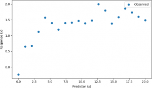
Machine learning techniques often rely on numerical values to control the learning (optimization) process. These parameters are known as hyperparameters. Hyperparameters differ from other parameters, such as weights in artificial neural networks, in that the latter are updated by the machine learning algorithm during training. Recall that machine learning algorithms generate a model. The parameters (as opposed to the hyperparameters) are specifically model parameters. Typical hyperparameters in ANNs are the number of hidden layers and/or the number of neurons in the hidden layer/layers, as this value is chosen by the user prior to ANN training. In other words, parameters are values for a model that the machine learning algorithm “learns”. Typically, the parameters that are learned results in a model that best fits observed data. For instance, suppose that several observations of a dependent variable (or response), say y, were collected at different times (the independent variable, or predictor variable), say x, and plotted on a scatter plot, as shown below (see).
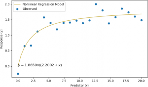
Suppose further that some information is known about the process that generated these observations. In other words, a model of the points is known. In this case, at a certain time (x), some value of an observation is recorded (y) according to a specific model, say, y = ax / (b + x). Finally, suppose that an algorithm, for instance, a machine learning algorithm, is used to estimate the values of a and b. In this case, a and b are the parameters of the model. The values used to control the machine learning algorithm are not part of the final model. These values are the hyperparameter values. Those hyperparameters are needed by the machine learning algorithm so that the parameters a and b can be estimated. For example, for the points above, the parameters were determined to be a = 1.86558 and b = 2.2002, so that the model is y = 1.86558x / (2.2002 + x). The model is a curved line, shown below in orange, that fits the observed points in blue.
Suppose that an ANN was used to “learn” a mapping between x and y in the example above. In this case, instead of the model parameters a and b, the model parameters may be weights on neurons (nodes) in the hidden layer that “map” the input x predictor variables to the output y response variables. The training data are the x values used as inputs, and the y values are the outputs, or labels. Then the hyperparameters include the number of hidden layers and the number of neurons in those hidden layers, the learning rate (a numerical value that is used during network training), and the maximum number of training iterations (generations), among other parameters that are not directly learned by the network, and that are not directly part of the model. Although, unlike the model parameters, the hyperparameters are not part of the model “learned” by the machine learning algorithm, the accuracy of the model depends heavily on the choice of hyperparameters.
For instance, selecting too many neurons in a hidden layer may result in an ANN that is too nonlinear, and it may have large fluctuations for values between the data points. An excessive number of training generations may result in the ANN being “overfit”, so that the network “memorizes” the mapping from the input (x) to the output (y), but it would not be able to “generalize”, or accurately values of x on which the network was not trained. The learning rate, used by the optimization (learning) algorithm, is another hyperparameter that is extremely important, especially in the context of ANNs. Learning rates that are too low may result in very slow training (or convergence) and stagnation during training (the network fails to improve with additional training iterations). A value too high may lead to premature convergence resulting in suboptimal model parameters, or an unstable training process. The learning rate hyperparameter is important in optimizing machine learning models, but the specific choice of the optimization algorithm itself is also a hyperparameter, and the user can select a technique from a number of different optimization options.
Different machine learning techniques, both supervised and unsupervised, employ different hyperparameters. As is the case with artificial neural networks and supervised learning, the performance of unsupervised machine learning algorithms is also heavily influenced by hyperparameters. As mentioned above, clustering is an important unsupervised learning method. The number of required clusters selected by the user is a hyperparameter.
Hyperparameter tuning is the user-driven process of selecting the hyperparameters that result in the best model. It is the process choosing the hyperparameters so that the machine learning algorithm learns the best parameters, thereby producing the best model. There are multiple approaches to select the correct value of a hyperparameter, or the best combination of values, in the case of more than one hyperparameter. A grid search is a straightforward approach for selecting parameters. A number of acceptable values are specified by the user for each hyperparameter, and combinations of these values are run, tested, and analyzed for accuracy and algorithm performance. For instance, in a machine learning method with two hyperparameters, the first having five values considered by the user to be important, and the second having eight such values, there are 40 different combinations that can be attempted. For a large number of hyperparameters, or for many possible values of each parameter, the number of combinations rapidly increases. For instance, in the case of four hyperparameters, if a user performs a grid search on ten values for each hyperparameter, there are 10,000 possible combinations. In most cases, however, the selection of one hyperparameter value will limit the values that make sense for the others, thereby decreasing the “search space” of the grid search.
Because of the importance of hyperparameter selection for the accuracy and performance of machine learning methods, hyperparameter tuning is an active research area in machine learning. Sophisticated techniques exist for selecting these values without having to perform a time-consuming exhaustive grid search. However, most implementations of machine learning algorithms, such as the Scikit Learn package in Python, supply suitable default values that result in good performance and accuracy. Users normally start hyperparameter tuning with these defaults and adjust some (or all) of the hyperparameters according to the specific application or by analyzing model results. Selecting the correct values for hyperparameters is still an inexact science. It is more of a craft. Machine learning practitioners develop skills in hyperparameter tuning with experience and with an in-depth knowledge and understanding of the algorithms involved in a particular machine learning approach.
THE IMPORTANCE OF THE HUMAN-IN-THE-LOOP
One way of considering the history of artificial intelligence is through “waves of enthusiasm”: periods of promise and heightened expectations and optimistic predictions of AI researchers about what could be achieved with AI (Brooks, 2021). Three waves of AI enthusiasm can be identified.
In the 1960s, research into symbolic computing, or logical reasoning with symbols instead of numbers, was predominant. Although artificial neural networks were introduced prior to that time (the pre-cursors to neural networks, perceptrons, were invented in 1957), AI experts generally rejected these type of connectionist models (neural networks consist of densely interconnected computing nodes, or neurons) in favour of symbolic computation. At the time, AI researchers predicted that human intelligence in computers was a decade away.
The second wave of enthusiasm occurred in the 1980s, with a new interest in neural networks generated by innovative learning algorithms, and with improvements in expert systems, which combined heuristics (general “rules of thumb”) with symbolic reasoning systems.
The third wave started in in the early 2000s, and continues to the present day, when new symbolic-reasoning systems were developed to solve difficult problems in Boolean logic (so-called 3SAT problems). Another major advance was successful applications of simultaneous localization and mapping (SLAM) for robotic-assisted building of maps as the robot collects information about its environment. This third wave was re-enforced when the availability of massive data sets resulted in major advances in artificial neural networks (Brooks, 2021).
Recall that the performance of supervised learning models (to which ANNs belong) is heavily dependent on having a large amount of training data. In this period, deep learning rose to prominence. In basic terms, deep learning refers to machine learning techniques with multiple layers. For instance, in ANNs, deep learning is implemented through multiple hidden layers.
In all these “waves of enthusiasm”, however, the successes of AI methods were due either humans guiding the process, or the cost of failure was very low. For instance, in safety-critical applications of machine learning, there was always human supervision, or a “human-in-the-loop”. Using AI to select advertisements to display on users’ web pages based on their browsing behaviours has been heralded in some quarters as a testimony to the success of machine intelligence. However, advertisements appearing that do not correspond with a user’s interest do not have major negative or damaging consequences. However, self-driving vehicles currently (as of 2022) require that a human be present and always have their hands on the steering wheel. Classification of people (e.g., determining credit risks) based on computational algorithms and flagging people as suspicious based on imperfect face-recognition technology are raise major ethical and social concerns (Brooks, 2021).
Another interesting example is speech understanding of entertainment and navigational systems, where human users adapt their own speech patterns to be better understood by the AI agent. In this case, the AI system seems to have “trained” its human user to communicate with it, instead of the other way around. Consequently, although there is a great amount of enthusiasm and optimism for new, innovative, and advanced artificial intelligence and machine learning techniques, human supervision, and, where necessary, intervention, is expected to be a necessity for the foreseeable future. The “human-in-the-loop” will remain a constant in AI, as it now seems unlikely that the former will surpass human intelligence for a long time to come (Brooks, 2021).
EXAMPLE OF SUPERVISED LEARNING AND STATISTICAL ANALYSIS IN LITERARY STUDIES
In the 20th century, there was clear demarcation between what “numbers” could represent, and what they could not.
It was generally assumed that numbers function best for measuring objective facts but could not capture the “infinite variation” of “human perception” that characterizes literary studies. Although the demarcation between these two areas was not always perfectly clear, machine learning has further weakened the boundary even further, as these methods are adaptive, and utilize examples for adaptation, rather than rigid quantitative measurements. They are therefore able to model aspects of the expertise of various academic communities. As a result, quantitative techniques are now sufficiently flexible to provide useful tools to literary historians and other digital humanities communities. The perspective has effectively shifted in the humanities from using “numbers” strictly for measurement to using them for broader purposes, such as modeling.
Of course, computational hardware is much faster, memory is much more expansive, and devices are much more seamless than in the early years of the digital humanities (or, as it was known previously, humanities computing). In addition, digital libraries are much larger and more easily accessible. Sophisticated processing and analysis algorithms, some of them leading-edge, others quite old, can now be efficiently run on inexpensive and readily available hardware. These factors have contributed to more widespread acceptance of quantitative methods in the digital humanities. Humanists are now beginning to think in terms of “models”, specifically statistical models. This blurring of the boundaries between “hard” quantitative measurements and the more perceptual interpretations of humanists is not entirely new. In the 1960s, Lotfi Zadeh proposed the idea of “fuzzy logic” that employs intervals instead of single measurements in an effort to model human decision-making.
In this context, machine learning has emerged as an effective approach to generating statistical, predictive models. In fact, as stated by Underwood, “The point of machine learning is exactly to model practices of categorization that lack a definition and can be inferred only from examples” (T. Underwood, 2020). And further, “[t]he goal of the inquiry is not to measure anything with inherent significance but rather to define a model – a relation between measurements – whose significance will come from social context (T. Underwood, 2020). It is important to emphasize that statistical models, like all approximations of complex realities, are imperfect, and therefore error analysis is also important for humanists.
Many of the machine learning algorithms used in the digital humanities are supervised learning in which the algorithm adapts from input (e.g., texts) that have been pre-classified, labeled, or annotated by humans.
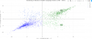
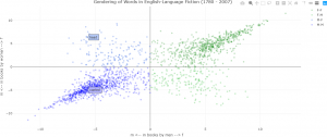
An example of the application of such models is interpreting perspectival differences and investigating the perspectival uses of machine learning. This research was part of a project to explore the changing significance of gender in fiction using a supervised approach. The research question was whether the prominence of gender in its characterization has varied from the end of the eighteenth century to the beginning of the twenty-first century (W. Underwood et al., 2018). Consequently, for the topic of “gender”, instead of attempting a definition of the term, a modeling approach may use a statistical analysis to generate a contrast between male and female perspectives on various words in literature that can be associated grammatically with male or female characters, categorized by male and female authors. That is, this statistical approach can be used to explore the divergence of two different perspectives on gender. A model developed and described in (W. Underwood et al., 2018) and (T. Underwood, 2020) demonstrates how words can be gendered. 87,800 works of fiction from 1780 to 2007 written in English were analyzed, resulting in an intuitive visualization to assess the results. The data are available HERE. Replication data are available HERE. Python code for implementing the model and generating several of the plots found in (W. Underwood et al., 2018) are available on HERE. In one task related to this research, classification was performed with a regularized logistic regression algorithm. There were 2200 features, obtained by optimizing 1600-character models on the entire collection. Each model had its own separate set of optimized hyperparameters (W. Underwood et al., 2018). A plot of words with gendered connotations then provides an indication of perspectival distortions (T. Underwood, 2020). Hovering over a point displays the word that is being represented. The x– and y zero axes are displayed by default, resulting in four quadrants. Each point is shown in a translucent colour to indicate density and clustering, and thus appear darker. The numeric values on the axes represents signed log likelihood ratio, which measures the goodness of fit in two competing models. Since the likelihood ratios can have a wide range of values for any analysis, the logarithms of the ratios are often used, as is the case here. A full mathematical development of this statistical text is beyond the scope of the current discussion. However, the plot has an intuitive interpretation. On each axis, positive values indicate that a particular word is overrepresented in descriptions of women, whereas negative numbers indicate that the word is overrepresented in descriptions of men. The northeast (x > 0, y > 0) and southwest (x < 0, y < 0) quadrants of the plot (books written by men describing feminine characteristics, and books written by women describing masculine characteristics, respectively) consist of words that have general agreement in gendered connotations. For example, the word “dress” appears in the northeast quadrant, indicating that the concept of “dress” is associated with female characters in both books written by men and by women. The word “pipe” appearing in the southwest quadrant indicates a strong association of “pipe” in male characters for both male and female authors (T. Underwood, 2020). Consequently, perceptual interpretation is straightforward while examining the southwest to northeast diagonal (moving upward left to right). However, when examining the northwest to southeast diagonal (moving downward left to right), it is seen that words in the northwest quadrant are those that men generally to apply to men, and that women tend to apply to women. This observation exhibits subjectivity in the perception of words, especially verbs (T. Underwood, 2020).
To generate the plot in Figure 1 in (T. Underwood, 2020), the following R code can be used. The code to generating the colourmap is found in the R script included with this section.
library(plotly)
## Read the data into a data frame.
data <-read.csv(²Data/genderedPerspectives_data4r.csv²)
##################################################
##
## Generate a colour map based on:
## [gender] mentioned in books by [gender]
##
## x => m
## y => f
##
##################################################
## Code to generate the colour map is found in the R script.
fig <- plot_ly(data = data, x = ~m, y = ~f, color = ~Written, colors = pal, text = ~word, hoverinfo = 'text', alpha = alpha)
fig <- fig %>% layout(title = 'Gendering of Words in English-Language Fiction (1780 - 2007)',
xaxis = list(title = 'm <-- in books by men --> f'),
yaxis = list(title = 'm <-- in books by women --> f')
)
## Display the figure.
fig
The resulting figure is shown below, showing overrepresented words describing female characters (top) and describing male characters (bottom) (T. Underwood, 2020).
The quantitative, machine learning approach to literary scholarship has many substantial critics, mostly on the grounds that quantitative measurements, as inherently objective, are not compatible with the (generally) more subjective approaches used in humanities scholarship. These critics fear that “numbers” are being used to replace the work of hermeneutics, or interpretation. However, as demonstrated in the example above, quantitative modeling techniques have appropriate applications to subjective, hermeneutic (interpretative) issues. For that reason, unsupervised methods in machine learning are de-emphasized. It is recalled that the example described above relies on supervised learning, with substantial human guidance in the form of labeling. Furthermore, novel machine learning and statistical modeling techniques are not always conceptually accessible to humanistic scholars. Very few of these scholars have advanced training in statistics, machine learning, or computational methods. Although well designed user interfaces and accessible and considered human-computer interaction can greatly assist humanists, including literary scholars, in using advanced modeling tools and drawing the correct insights from them, these scholars will need to possess a more-than-basic knowledge of statistics, and have more than a passing familiarity with programming – although programming languages most favoured by humanists, such as Python and R, greatly simplify the task. As Underwood states, “[a] discipline not trained to use statistical models will necessarily see them as foreign competition” (T. Underwood, 2020).
