Working with Data
8 Further Adventures in Data Cleaning: Working with Data in Excel and R
Dr. Rong Luo and Berenica Vejvoda
Learning Outcomes
By the end of this chapter you should be able to:
- Explain general procedures for preparing for data cleaning.
- Perform common data cleaning tasks using Excel.
- Import data and perform basic data cleaning tasks using the R programming language.
Introduction
Data cleaning is an essential part of the research process. In the previous chapter, you were introduced to some common, basic data cleaning tasks. In this chapter, we will delve more deeply into data exploration, manipulation, and cleaning using some flexible general-purpose research tools. The tools that we highlight are, in some cases, the same tools researchers use for analyzing their data, and it’s helpful for curators and data managers to be familiar with them.
General Procedures to Prepare for Data Cleaning
Without preparation before the data cleaning process, you may run into critical issues such as data loss. In this section, we will discuss general steps that you should take before the data cleaning process.
Making a Backup
Research data management (RDM) practices recommend creating secure backups of your data to ensure that if it is incorrectly altered during the cleaning process, the original data can always be restored. This backup copy of the original data should not be modified in any situation. You should also keep a record/log of the changes you make. You would be surprised by how many researchers create errors in their original data while they are trying to “improve” it. If a data analyst needs to access the original data, you should either send or share a copy of the data or allow read-only access to the original data.
Understanding the Data
The first step in cleaning data is understanding the data that is being cleaned. To understand the data, begin by doing some basic data exploration (or Exploratory Data Analysis) and get a sense of what problems, if any, exist within the data. Check the data values against their definitions in the metadata file or documentation for issues such as out-of-range or impossible values (e.g., negative age or age over 200). Ensure you have and understand workable data column names. Check delimiters that separate values in text files and ensure your data values don’t embed the delimiter itself. If you didn’t number your observations, you should add a unique record number to individual observations within the dataset so that you can easily find problem records by referencing that number.
Planning the Cleaning Process
Data cleaning must be done systematically to ensure all data is cleaned using the same procedures. This ensures data integrity and allows data to be easily processed during analysis. To create a plan for cleaning a specific field in a dataset, ask yourself the following three questions:
- What is the data you are cleaning?
- How will you identify an issue within the dataset that should be cleaned?
- How should it be cleaned?
Choosing the Right Tools
One of the most important stages of data cleaning is choosing the right tool for a specific purpose. The previous chapter highlighted OpenRefine, a handy, special-purpose data-cleaning tool. Here, we discuss Excel and R, two powerful, general-purpose software tools, and highlight a few of the data cleaning features of each.
Data Cleaning Tools
The data cleaning tool you choose will depend on factors including your computing environment, your level of programming expertise, and your data readiness requirements. You have a wide variety of software and methods to choose from for cleaning and transforming data. We’ll review Excel/Google Sheets and R programming language.
Microsoft Excel/Google Sheets
Excel and Google Sheets are great tools for data cleaning and contain a variety of built-in automated data cleaning functions and features. Excel is widely available for both Windows and MacOS as a desktop program, and Google Sheets is available online. They are similar and easy to learn, use, and understand. They can both import and export the commonly used CSV data file format and other common spreadsheet formats. When exporting, be sure to check the exported data column names for usability, as some statistical packages will have issues if column names contain embedded spaces or special characters. Common data cleaning techniques used in Excel and Google Sheets for editing and manipulation are summarized in the Function table below.
| Function | Description |
| = CONCATENATE | Combines multiple columns |
| = TRIM | Removes all spaces from a text string except for single spaces between words |
| = LEFT | Returns the first character or characters in a text string, based on the number of characters you specify |
| = RIGHT | Returns the last character or characters in a text string, based on the number of characters you specify |
| = MID | Returns a specific number of characters from a text string, starting at the position you specify, based on the number of characters you specify |
| = LOWER | Converts a text string to all lower case letters |
| = UPPER | Converts a text string to all upper case letters |
| = PROPER | Converts a text string to proper case so that the first letter in each word is upper case and all other letters are lower case |
| = VALUE | Converts text string to numeric |
| = TEXT | Converts numbers to text |
| = SUBSTITUTE | Replaces specific text in a text string |
| = REPLACE | Replaces part of a text string, based on the position and number of characters specified, with a different text string |
| = CLEAN | Removes all non-printable characters from a text string |
| = DATE | Returns the number that represents the date in Microsoft Excel date-time code |
| = ROUND | Rounds a selected cell to a specified number of digits |
| = FIND | Returns the starting position of one text string within another text string. FIND is case-sensitive |
| = SEARCH | Returns the number of the starting position of a specific character or text string within another text string, reading left to right (not case-sensitive) |
To understand some of these functions, we will consider a number of common errors seen in imported data, including line breaks in the wrong place, extra spaces or no spaces in and between words, improperly capitalized or all upper case/lower case text, ill-formatted data values, and non-printing characters.
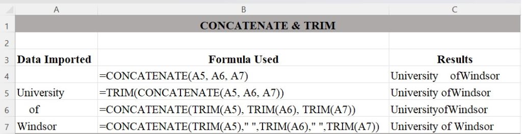
Figure 1 illustrates combinations of CONCATENATE and TRIM nested in various ways to find the best output configuration for how you want the text to appear.[1] It is an example of how you can generate a single line of text from the contents of three rows by nesting two Excel functions. CONCATENATE will merge the three cells into one, but it does nothing about the extra spaces you see in the text. TRIM will remove all spaces except for single spaces between words, but it won’t add needed spaces, so we need to add quotation marks for Excel to add the needed blank spaces in between words.
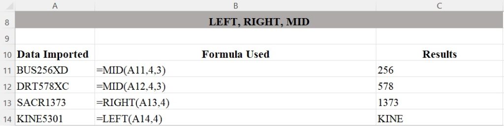
The LEFT, RIGHT, and MID functions in Figure 2 demonstrate how to process data from certain directions depending on where the text or number you wish to extract are in the string.
Rows 11 and 12 show how to use the MID function to extract numbers from the middle of a text string. The MID function takes three arguments: a reference to the string you’re working with, the location of the first character you want to extract, and the number of characters you want to extract. So MID(A11,4,3) first looks up the contents of cell A11 and finds the string “BUS256XD,” and then returns three characters starting with the fourth character: 256. The data in C11 and C12 are the results of using the MID function in rows 11 and 12.
The LEFT and RIGHT functions only take two arguments: the string and the starting point. These functions then return the rest of the string, going either left or right. C13 and C14 show portions of course numbers that have been extracted from A13 and A14 using the RIGHT and LEFT functions.
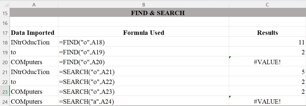
Figure 3 illustrates the difference between FIND and SEARCH. The FIND function in Excel is used to return the position of a specific character or substring within a text string and is case sensitive. The SEARCH function in Excel also returns the location of a character or substring in a text string. Unlike FIND, the SEARCH function is not case sensitive. Both FIND and SEARCH return the #VALUE! error if the specific character or substring does not exist within the text.
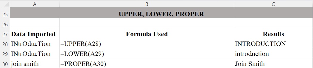
Figure 4 shows how the UPPER, LOWER, and PROPER functions are used to produce the contents for data. The UPPER function changes all text to upper case. The LOWER function changes all text to lower case. The PROPER function changes the first letter in each word to upper case and all other letters to lower case, which is useful for fixing names.
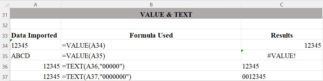
Excel aligns strings in a column based on how they are stored: text (including numbers that have been stored as text) are left aligned, numbers are right aligned. In Figure 5, the VALUE function converts text that appears in a recognized format (such as a numbers, dates, or time formats) into a numeric value. If text is not in one of these formats, VALUE returns the #VALUE! error. The TEXT function lets you change the way a number appears by applying format codes, which is useful in situations where you want to display numbers in a more readable format. But keep in mind that Excel now “thinks” of the number as text, so running calculations on it may not work or may lead to unexpected results. It’s best to keep your original value in one cell, then use the TEXT function to create a formatted copy of the number in another cell.
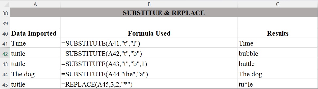
Figure 6 illustrates how the SUBSTITUTE function replaces one or more text strings with another text string. This function is useful when you want to substitute old text in a string with a new string. However, it is not case sensitive. For example, in cell A41, the function will not substitute “t” for the “T” in “Time”. There is a difference between the SUBSTITUTE and the REPLACE functions. You can use SUBSTITUTE when you want to replace specific characters wherever they occur in a text string, and you can use REPLACE when you want to replace any text that occurs in a specific location in a text string.
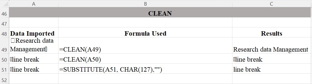
The CLEAN function shown in Figure 7 removes non-printable characters, such as carriage returns (↩) or other control characters, represented by the first 32 codes in 7-bit ASCII code from the given text. Data imported from various sources may include non-printable characters and the CLEAN function can help remove them from a supplied text string. In Excel, a non-printing character may show up as a box symbol (☐). Note that the CLEAN function lacks the ability to remove all non-printing characters (e.g., “delete character”). You can specify an ASCII character using the Excel function CHAR and the number of the ASCII code. For example CHAR(127) is the delete code. To remove a non-printing character, you can simply substitute the offending non-printable character with nothing enclosed in quotation marks (“”).
The exercise below shows the CHAR(19) non-printing character in row 10, which looks like “!!”.
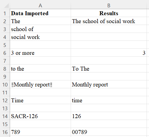
Exercise 1
Generate the cleaning results in column B from data imported in column A by using Excel/Google Sheets functions.
View Solutions for answers.
R Programming Language
While spreadsheet software like Excel and Google Sheets provide common functions that can assist with data cleaning, it can be very difficult to use them to work with larger datasets. Additionally, if Excel or Google Sheets do not have a specific built-in function, you will require a considerable amount of programming to build that function. The R program can help. R is one of the most well-known, freely available statistical software packages that can be used in the data cleaning process. R is a fully functional programming language with features for working with statistics and data, but you don’t need to know how to program to use some basic functions.
The two most important components of the R language are objects, which store data, and functions, which manipulate data. R also uses a host of operators like +, -, *, /, and <- to do basic tasks. To work with R you type commands at a prompt, represented by “>”.
To create an R object, choose a name and then use the less-than symbol followed by a minus sign to save data into it. This combination looks like an arrow, <-. For example, you can save data “1” into an object “a”. Wherever R encounters the object “a,” it will replace it with the data “1” saved inside, like so:
> a <- 1
R comes with many functions that you can use to do sophisticated tasks. For example, you can round a number with the round function. Using a function is pretty simple. Just write the name of the function and then the data you want the function to operate on in parentheses:
> round (3.1415)

[1] 3
R packages are collections of functions written by R’s developers. You may need to install other packages (dependencies, packages that other packages are dependent on) up front to get it to work. It is easier to just set up dependencies = TRUE when you install R packages.
> install.packages(“package name”, dependencies = TRUE)
Let’s begin with downloading and installing the required software. R is available for Windows, MacOS, and Linux.
1. Install R and RStudio
R can be downloaded here: https://cran.rstudio.com/.
- For Windows users, https://cran.rstudio.com/bin/windows/base/.
- For Mac users, https://cran.rstudio.com/bin/macosx/.
- For Linux users, https://cran.r-project.org/bin/linux/.
Base R is simply a command-line tool: you type in commands at a prompt and see the results displayed on the screen. RStudio, on the other hand, is an integrated development environment (IDE), a set of tools including a script editor, a command prompt, and a results window, as well as some menu commands for commonly used R functions. When people talk about working in R, they usually mean using R through RStudio. Please note that to use RStudio you will need to install R first.
Download and install RStudio Desktop, which is also free and available for Windows, Mac, and various versions of Linux here: https://posit.co/download/rstudio-desktop/.
2. Become familiar with RStudio
Before importing any data, you want to become familiar with RStudio.
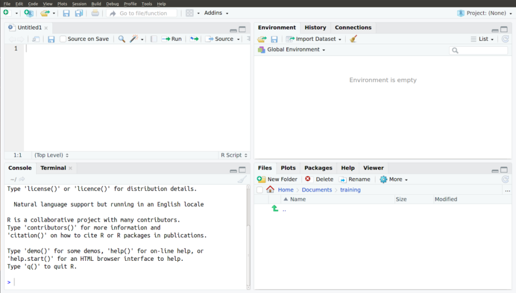
The R studio has four quadrants (see Figure 8):
| Section | Purpose |
| Top Left | This section shows you the script(s) you are currently editing. An R script is a set of R commands and comments. They are commonly used to keep of track of the commands that need to be run and provide explanatory notes on the purpose of the commands through comments. |
| Top right | The “Environment” tab lists all the variables and functions defined and used in a session. |
| The “History” tab lists all the commands typed in the R Console (bottom left of RStudio). | |
| The “Connections” tab can help you connect to an external database to access data that is not on your local computer. | |
| Bottom left | The “Console” tab displays a command prompt to allow you to use R interactively, just like you would without RStudio. |
| The “Terminal” tab opens a system shell to perform advanced functions, such as accessing a remote system. | |
| Bottom right | The “Files” tab lets you keep track of, open, and save files associated with your R project. |
| The “Plots” tab shows graphs being plotted. | |
| The “Packages” tab allows you to load and install packages to add additional R functions. | |
| The “Help” tab provides useful information about some functions. | |
| The “Viewer” tab can be used to view and interact with local web content. |
You can type R commands in the console at a prompt, just as you would if you were working without RStudio. You can then view the results in the “History” and “Environment” tabs. Your work is not automatically saved when R is closed. You can copy and paste your console to a text file to save it.
For example, you can open RStudio and type the following command in the console (the text after the prompt “>”):
> print("Hello")
R will return the following output:
[1] "Hello"
In addition to working interactively by typing commands at the prompt, you can also create R script files using the RStudio editor shown in the top right quadrant. Script files are text files containing a sequence of R commands that can be run one after another. You can select your commands in the script files and run them one at a time or all together. Writing and saving your commands for data cleaning in a script file allows you to better track your work, and you can more easily rerun code later and across new datasets. Tracking your work in this way is a good RDM practice.
Open a new script by selecting the top left icon:
![]()
Before importing your dataset, you should set your working directory to the dataset’s location. From RStudio, use the menu to change your working directory to the directory where you saved the sample data file. In the “Session” menu, choose > Set Working Directory > Choose Directory.
Alternatively, in the console window (or script editor), you can use the R function setwd(), which stands for “set working directory”. Forward slashes (/), rather than backslashes, are in the path. So, if you saved the data to “C:\data”, you would enter the command:
> setwd("C:/data")
3. Importing data
You can import data in different formats using R. CSV files are commonly used for numeric data. While they look like standard Excel files, they are simply text files with columns separated by commas. You can export CSV data from Excel using “save as,” and it is commonly used as a preservation format for data management, as it can be read by many programs.
For the next set of examples, we are going to be working with a sample dataset, sample.csv, that is available in Borealis. Please download and save this dataset to a new folder on your computer. The SPSS and Excel files needed for these examples are also available in Borealis.
To load the CSV file, first create a new script file in the script editor. Type the following command in the script to use R’s built-in read.csv command, and then run the script.
> mydata_csv<-read.csv("sample.csv")
The default delimiter of the read.csv() function is a comma, but if you need to read a file that uses other delimiters, you can do so by supplying the “sep” argument to the function (e.g., adding sep = ‘;’ allows a semi-colon separated file).
> mydata_csv<-read.csv(“sample.csv”, sep=’;’)
Please note that “mydata_csv” in the above command refers to the object (data frame) that will be created when the read.csv function imports the file “sample.csv”. Think of the “mydata_csv” data frame as the container R uses to hold the data from the CSV file.
R commands follow a certain pattern. Let’s go through this one from right to left. In above command, mydata_csv<-read.csv(“sample.csv”, sep=’;’), read.csv is a function to read in a CSV file and has two parameters. The first, sample.csv, tells read.csv what file to read in, while the second, sep=’;’, tells it that the data points in the file are separated by semi-colons. After read.csv parses the file, the assignment operator, <-, assigns the data to mydata_csv, which is an object (data frame) created to hold the data. You can now use and manipulate the data in the data frame.
In R, <- is the most common assignment operator. You can also use the equal sign, =. For more information, use the help command, which is just a question mark followed by the name of the command:
> ?read.csv
To read in an Excel file, first download and install the readxl package. In the R console, use the following command:
> install.packages("readxl")
Please note that sometimes packages are dependent on other associated packages to function properly. By using existing packages, programmers can save time when creating new functionalities by using existing functions that were already implemented. However, it may be difficult to figure out if a package requires another package to function. As such, it is good practice to install packages by including the dependencies statement (TRUE tells R the dependencies should be included). By setting the dependencies parameter to TRUE, we tell R to also download and install all the required packages needed by the package that we are trying to install.
> install.packages(“readxl”, dependencies = TRUE)
After the package downloads and installs, use the library() function to load the readxl package.
> library(readxl)
Note that with the library function, unlike the install.package function, you do not put the name of the package in quotes.
Now you can load the Excel file with the read_excel() function:
> mydata_excel <- read_excel("sample.xlsx")
For more information, use the ?read_excel help command.
Statistical Package for the Social Sciences (SPSS) SAV files can be read into R using the haven package, which adds additional functions to allow importing data from other statistical tools.
Install haven by using the following command:
> install.packages("haven", dependencies = TRUE)
After the package downloads and installs, use the library() function to load the package:
> library(haven)
Now you can load the SPSS file with the read_sav() function:
> mydata_spss <- read_sav("sample.sav")
You can import SAS and Stata files too. For more information, use the ?haven or ?read_sav help commands, or visit the https://haven.tidyverse.org/.
Data can also be loaded directly from the internet using the same functions as listed above (except for Excel files). Just use a web address instead of the file path.
> mydata_web <- read.csv(url("http://some.where.net/data/sample.csv"))
Now that the data has been loaded into R, you can start to perform operations and analyses to investigate any potential issues.
4. Inspecting data
R is a much more flexible tool for working with data than Excel. We will cover the most basic R functions for examining a dataset.
Assume that the following text file with eight rows and five columns is stored as sample.csv.
1,4.1,3.5,setosa,A
2,14.9,3,set0sa,B
3,5,3.6,setosa,C
4,NA,3.9,setosa,A
5,5.8,2.7,virginica,A
6,7.1,3,virginica,B
7,6.3,NA,virginica,C
8,8,7,virginica,C
Now consider the following command to import data. Since the dataset does not contain a header (that is, the first row does not list the column names), you should specify header=FALSE. If you want to manually set the column names, you specify the col.names argument. In the command below, we asked read.csv to set the column names to ID, Length, Width, Species, and Site. Using colClasses, we can specify what data type (number, characters, etc.) we expect the data contained in the columns to be. In this case, we have specified to read.csv that it should treat the first and last two columns as factor (categorical data) and the middle two columns as numeric (numbers).
Enter the following command into your script editor and run it:
> mydata_csv <- read.csv("sample.csv", header = F, col.names = c("ID","Length", "Width", "Species", "Site"), colClasses=c("factor","numeric","numeric","factor", "factor"))
The data is now loaded into mydata_csv. To view the data we loaded, run the following line:
> mydata_csv
R will return the data from the file it’s read in.
ID Length Width Species Site
1  1    4.1   3.5    setosa    A
2  2   14.9   3.0    set0sa    B
3  3    5.0   3.6    setosa    C
4  4     NA   3.9    setosa    A
5  5    5.8   2.7 virginica    A
6  6    7.1   3.0 virginica    B
7  7    6.3    NA virginica    C
8  8    8.0   7.0 virginica    C
The output above shows five columns of data. The first column specifies the row number and is automatically created by R when the data is loaded. The first row displays the column names that we have specified.
One of the first commands to run after loading the dataset is the dim command, which prints out the dimensions of the loaded data by row and column. This command allows you to verify that all entries have been correctly read by R. In this case, the sample dataset should have eight entries with five columns. Let’s run dim to see if all the data are loaded.
> dim(mydata_csv)
After running the command above, R will output the following:
[1] 8 5
The output tells us that there are eight rows and five columns in the loaded data. This matches our expectation, so all the data have been loaded.
You can also run the summary command, which gives some basic information about each column in the dataset. The summary command returns the maximum and minimum values, the lower and upper quartiles (the lower quartile is the value below which 25% of the data in a dataset fall and the upper quartile is the value above which 75% of the data in a dataset fall), and the median for numeric columns and the frequency for factor columns (the number of times each value appears in a column).
> summary(mydata_csv)
      ID        Length           Width            Species  Site
 1      :1   Min.   : 4.100   Min.   :2.700   set0sa   :1   A:3
 2      :1   1st Qu.: 5.400   1st Qu.:3.000   setosa   :3   B:2
 3      :1   Median : 6.300   Median :3.500   virginica:4   C:3
 4      :1   Mean   : 7.314   Mean   :3.814
 5      :1   3rd Qu.: 7.550   3rd Qu.:3.750
 6      :1   Max.   :14.900   Max.   :7.000
 (Other):2   NA's   :1        NA's   :1
From the output, we can see that there are five columns. Since we asked R to read the “Length” and “Width” columns as numeric, it calculated and displayed summary information about the numbers in those columns, such as the minimum, maximum, mean, and quartiles. The information about each column is displayed in rows under the column’s name. For example, in the “Length” column, you can see that the minimum value is 4.1, and the maximum is 14.9. The 1st Qu. shows the lower quartile, which is 5.4, and the 3rd Qu. shows the upper quartile, which is 7.55.
The NA’s row tells us if there are any missing values. In R, missing values are represented by the symbol NA (not available). From the summary output, there are two missing data: one in the “Length” column and one in the “Width” column.
In the “Species” column, which was read in as factors (or categories), each of the rows displays the frequency with which a value appears in the column. From the output, we can see that there are three instances of setosa, four of virginica, and one of set0sa.
Here it is possible to identify recording errors. Instead of setosa, there is one flower mistakenly entered as set0sa. This kind of typo is very common when recording data, but it’s very difficult to find since zero and the letter “o” appear very similar in most fonts.
R uses a basic function, is.na, to test and list whether data values are missing. This function returns a value of true and false for each value in a dataset. If the value is missing, the is.na function returns a value of “TRUE,” otherwise, it will return a value of ”FALSE.”
> is.na(mydata_csv$Length)

[1] FALSE FALSE FALSE TRUE FALSE FALSE FALSE FALSE
Note that the dollar sign ($) is used to specify columns. In this case we are investigating if the column “Length” in the CSV dataset contains missing values. As you can see from the output, there is one missing value, so the function returns “TRUE” for that entry in the column.
Outliers are data points that dramatically differ from others in the dataset and can cause problems with certain types of data models and analysis. For instance, an outlier can affect the mean by being unusually small or unusually large. While outliers can affect the results of an analysis, you should be cautious about removing them. Only remove an outlier if you can prove that it is erroneous (i.e., if it is obviously due to incorrect data entry). One easy way to spot outliers is to visualize the data items’ distribution. For example, type the following command, which is asking R to generate a boxplot.
boxplot(mydata_csv$Length)
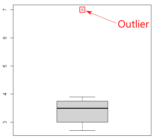
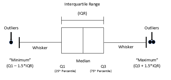
Boxplots are useful for detecting potential outliers (see Figure 9). A boxplot helps visualize a quantitative column by displaying five common location summaries: minimum, median, first and third quartiles (Q1 and Q3), and maximum. It also displays any observation that is classified as a suspected outlier using the interquartile range (IQR) criterion, where IQR is the difference between the third and first quartile (see Figure 10). An outlier is defined as a data point that is located outside the whiskers of the boxplot. In the above boxplot output, the circle at the top represents a data point that is very far away from the rest of the data, which are mostly contained in the “box” of the plot.
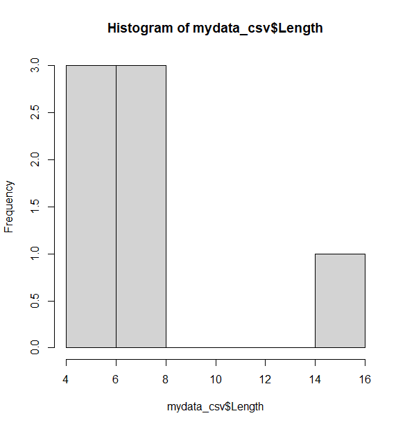
Another basic way to detect outliers is to draw a histogram of the data. A histogram shows the distribution of the different values in the data. From the histogram below, it appears there is one observation that is higher than all other observations (see the bar on the right side of the plot), which is consistent with the boxplot. The following command will generate a histogram:
> hist(mydata_csv$Length)
> summary(mydata_csv$Length)
Min. 1st Qu. Median Mean 3rd Qu. Max. NA's
4.100 5.400 6.300 7.314 7.550 14.900 1
From the summary output, one value, 14.90, for length seems unusually large, although not impossible according to common sense. This requires further investigation. Such outliers can significantly affect data analysis, so it’s important to understand their validity. Removing outliers must be done carefully since outliers can represent real, meaningful observations rather than recording errors.
Now that we have done some preliminary inspection on the raw data, suppose the raw data have several issues that need to be fixed. These issues include:
- Redundant “Site” column
- Typo in the “Species” column
- Missing values in the “Length” and “Width” columns
- Outlier in the “Length” column
With these issues in mind, we can move on to the next stage and start cleaning the data.
5. Cleaning the data
First, let’s start by dropping an extra column. Using the data above, suppose we want to drop the “Site” column. As seen in the output of the summary command, “Site” is the fifth column in the dataset. To drop this, we can run the following command:
> mydata_csv <- mydata_csv[-5]
The above command uses the square brackets to specify the columns of the original data. By using a negative number, we tell R to retrieve all columns except for the specified column. In this case, the “Site” column is the fifth column. Since we want to remove the fifth column but keep all other columns, we can use -5 in the square brackets to tell R to fetch all columns except for the fifth column. Then, by reassigning the new data that we fetched to mydata_csv, we’ve effectively deleted the fifth column.
To verify that the column has been successfully removed, we can use the dim command, as seen before.
> dim(mydata_csv)
[1] 8 4
From the output, we can see that the data has four (versus five) columns now.
Next, it’s time to clean the typos. In this case, since you know that the typo is set0sa and it should actually be setosa, you can replace all matching cells using the following command:
> mydata_csv[mydata_csv=="set0sa"] = "setosa"
> summary(mydata_csv)
ID Length Width Species
1 :1 Min. : 4.100 Min. :2.700 set0sa :0
2 :1 1st Qu.: 5.400 1st Qu.:3.000 setosa :4
3 :1 Median : 6.300 Median :3.500 virginica:4
4 :1 Mean : 7.314 Mean :3.814
5 :1 3rd Qu.: 7.550 3rd Qu.:3.750
6 :1 Max. :14.900 Max. :7.000
(Other):2 NA's :1 NA's :1
Note that the equality operator, “==”, selects all instances of “set0sa” (in this case, one instance) and “=” assigns it to be “setosa”. Using two equals signs to test for equality and a single equals sign to set something equal to something else is a common programming convention.
You can see that there are now zero entries in the “Species” column with the name set0sa from the summary() output. The data have been cleaned for this typo.
There are several ways to deal with missing data. One option is to exclude missing values from analysis. Prior to removing NA from the “Length” column, the mean() function returns NA as follows:
> mean(mydata_csv$Length)
[1] NA
This is done because it is impossible to use NA in a numeric analysis. Using na.rm to remove the missing value NA returns a mean of 7.314286:
> mean(mydata_csv$Length, na.rm = T)

[1] 7.314286
Exercise 2
Check if there are any outliers in the “Width” column of sample.csv by using a boxplot, then calculate the mean of length by removing the outliers.
View Solutions for answers.
Conclusion
Data cleaning procedures are important foundations for successful data analysis and should be performed before analyzing data. In this chapter, we have only scratched the surface of data cleaning issues and fixes that researchers need in order to create clean data using Excel/Google Sheets and R language. Extensive libraries of data manipulation functions exist, and they offer functionalities that might help you in your data cleaning process. Additional R documentation can be found at the following sites: https://cran.r-project.org/manuals.html and https://cran.r-project.org/web/packages/available_packages_by_name.html.
Key Takeaways
- General procedures in preparing for data cleaning are making a backup, understanding the data, planning the cleaning process, and choosing appropriate tools.
- Excel functions can be used to perform many basic data cleaning tasks.
- The R programming language is a useful and free software package that can be used for more advanced cleaning procedures.
Acknowledgment
The authors thank Kristi Thompson and other editors whose constructive comments have improved this chapter.
the process of employing six core activities: discovering, structuring, cleaning, enriching, validating, and publishing data.
a term that describes all the activities that researchers perform to structure, organize, and maintain research data before, during, and after the research process.
a process used to explore, analyze, and summarize datasets through quantitative and graphical methods. EDA makes it easier to find patterns and discover irregularities and inconsistencies in the dataset.
data about data; data that define and describe the characteristics of other data.
special characters reserved by computational systems or languages to denote independent objects or elements.
an open source data manipulation tool that cleans, reshapes, and batch edits messy and unstructured data.
a delimited text file that uses a comma to separate values within a data record.
the values or variables that are provided to the function.
a data structure that contains a set of values of a particular type. R objects can be created, modified, and used to perform computations and analyses.
a computer program that can be run from the command line interface (CLI) of an operating system. The CLI is a text-based interface that allows the user to interact with the computer using typed commands, instead of using a graphical user interface (GUI) with menus and icons.
a software application that provides a comprehensive environment for software development. RStudio is an integrated development environment (IDE) that enables users to write, debug, run R code and display the corresponding outputs.
text files containing a sequence of R commands that can be run one after another
the values that divide a list of numbers into quarters.
data points which dramatically differ from others in the dataset and can cause problems with certain types of data models and analysis.
also known as a box-and-whisker plot, a boxplot is a graphical representation of a dataset that displays the distribution of the data and any potential outliers.
a graphical representation of the distribution of a set of continuous or discrete data.
