Working with Data
7 Data Cleaning During the Research Data Management Process
Lucia Costanzo
Learning Outcomes
By the end of this chapter you should be able to:
- Describe why it is important to clean your data.
- Recall the common data cleaning tasks.
- Implement common data cleaning tasks using OpenRefine.
What Is Data Cleaning?
You may have heard of the 80/20 dilemma: Most researchers spend 80% of their time finding, cleaning, and reorganizing huge amounts of data and only 20% of their time on actual data analysis.
When starting a research project, you will use either primary data generated from your own experiment or secondary data from another researcher’s experiment. Once you obtain data to answer your research question(s), you’ll need time to explore and understand it. The data may be in a format which will not allow for easy analysis. During the data cleaning phase, you’ll use Research Data Management (RDM) practices. The data cleaning process can be time consuming and tedious but is crucial to ensure accurate and high-quality research.
Data cleaning may seem to be an obvious step, but it is where most researchers struggle. George Fuechsel, an IBM programmer and instructor, coined the phrase “garbage in, garbage out” (Lidwell et al, 2010) to remind his students that a computer processes what it is given — whether the information is good or bad. The same applies to researchers; no matter how good your methods are, the analysis relies on the quality of the data. That is, the results and conclusions of a research study will be as reliable as the data that you used.
Using data that have been cleaned ensures you won’t waste time on unnecessary analysis.
Six Core Data Cleaning and Preparation Activities
Data cleaning and preparation can be distilled into six core activities: discovering, structuring, cleaning, enriching, validating, and publishing. These are conducted throughout the research project to keep data organized. Let’s take a closer look at these activities.
1. Discovering Data
The important step of discovering what’s in your data is often referred to as Exploratory Data Analysis (EDA). The concept of EDA was developed in the late 1970s by American mathematician John Tukey. According to a memoir, “Tukey often likened EDA to detective work. The role of the data analyst is to listen to the data in as many ways as possible until a plausible ‘story’ of the data is apparent” (Behrens, 1997). EDA is an approach used to better understand the data through quantitative and graphical methods.
Quantitative methods summarize variable characteristics by using measures of central tendency, including mean, median, and mode. The most common is mean. Measures of spread indicate how far from the center one is likely to find data points. Variance, standard deviation, range, and interquartile range are all measures of spread. Quantitatively, the shape of the distribution can be evaluated using skewness, which is a measure of asymmetry. Histograms, boxplots, and sometimes stem-and-leaf plots are used for quick visual inspections of each variable for central tendency, spread, modality, shape, and outliers.
Exploring data through EDA techniques supports discovery of underlying patterns and anomalies, helps frame hypotheses, and verifies assumptions related to analysis. Now let’s take a closer look at structuring the data.
2. Structuring Data
Depending on the research question(s), you may need to set up the data in different ways for different types of analyses. Repeated measures data, where each experimental unit or subject is measured at several points in time or at different conditions, can be used to illustrate this.
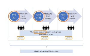
In Figure 1, researchers might be investigating the effect of a morning breakfast program on Grade 6 students and want to collect test scores at three time points, such as the pre- (T1), mid- (T2), and post-morning (T3) periods of the breakfast program. Note that the same students are in each group, with each student being measured at different points in time. Each measurement is a snapshot in time during the study. There are two different ways to structure repeated measures data: long and wide formats.
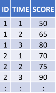
Table 1 shows data structured in long format, with each student in the study represented by three rows of data, one for each time point for which test scores were collected. Looking at the first row, Student One at Timepoint 1 (before the breakfast program) scored 50 on the test. In the second row, Student One at Timepoint 2 (midway through the breakfast program) scored higher on the test, at 65. And in the third row, Student One at Timepoint 3 (after the program) scored 80.
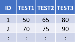
The wide format, shown in Table 2, uses one row for each observation or participant, and each measurement or response is in a separate column. In wide format, each student’s repeated test scores are in a row, and each test result for the student is in a column. Looking at the first row, Student One scored 50 on the test before the breakfast program, then scored 65 on the test midway through the breakfast program, and achieved 80 on the test after the program.
So, a long data format uses multiple rows for each observation or participant, while wide data formats use one row per observation. How you choose to structure your data (long or wide) will depend on the model or statistical analysis you’re undertaking. It is possible you may need to structure your data in both long and wide data formats to achieve your analysis goals.
Structuring is an important core data cleaning and preparation activity that focuses on reshaping data for a particular statistical analysis. Data can contain irregularities and inconsistencies, which can impact the accuracy of the researcher’s models. Let’s take a closer look at cleaning the data, so that your analysis can provide accurate results.
3. Cleaning Data
Data cleaning is central to ensuring you have high-quality data for analysis. The following nine tips address a range of commonly encountered data cleaning issues using practical examples.
Tip 1: Spell Check
 Finding misspelled words and inconsistent spellings is one of the most important data cleaning tasks. You can use a spell checker to identify and correct spelling or data entry errors.
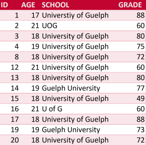
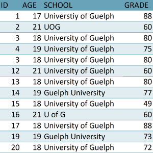
Spell checkers can also be used to standardize names. For example, if a dataset contained entries for “University of Guelph” and “UOG” and “U of G” and “Guelph University” (Table 3), each spelling would be counted as a different school. It doesn’t matter which spelling you use, just make sure it’s standard throughout the dataset.
Tip 01 Exercise: Spell Check
Go through Table 3 and standardize the name as “University of Guelph” in the SCHOOL column.
View Solutions for answers. Data files for the exercises in this chapter are available in the Borealis archive for this text.
Tip 2: Duplicates
 Sometimes data have been manually entered or generated using methods that could cause duplications of rows. Check rows to determine if data have been duplicated and need to be deleted. If each row has an identification number, it should be unique for each observation. In this example, there are two observations with an ID number of 3 (Table 4) and both have the same values, so one of these rows of data should be deleted.
Tip 02: Exercise: Duplicates
Go through Table 4 and delete the duplicate observations.
HINT: If using Excel, look for and use the ‘Duplicate Values’ feature.
View Solutions for answers.
Tip 3: Find and Replace
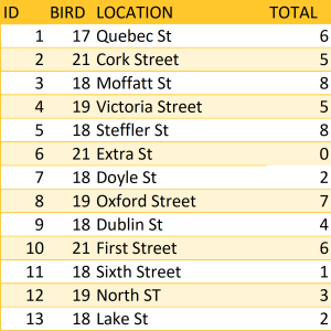
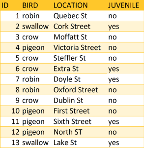
 With some carefully crafted replacements, it’s possible to get data fairly clean and into a good format by looking for patterns and repetition in a file. In this example, we’re counting the number of bird sightings in Guelph. Looking at the LOCATION column, we need to replace the abbreviations “St” and “ST” with the full spelling of “street” (Table 5). This can be done using the basic Find and Replace function.
Tip 03 Exercise: Find and Replace
Go through Table 5. Find and replace all instances of “ST” and “st” with “Street” in the LOCATION column.
HINT: Use caution with global Find and Replace functions. In the example shown below, instances of ‘St’ or ‘st’ that do NOT indicate ‘Street’ (e.g. ‘Steffler’ and ‘First’) will be erroneously replaced. Avoid such unwanted changes by strategically including a leading space in the string you are searching for (so, ‘spaceSt’). Experiment with the ‘match case’ feature as well, if available. Always keep a backup of your unchanged data in case things go awry.
View Solutions for answers.
Tip 4: Letter Case
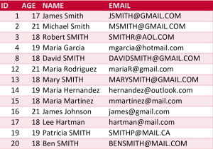
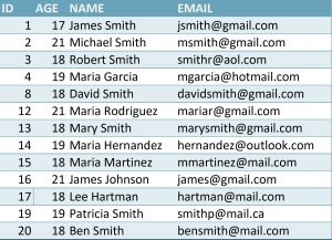
 Text may be lowercase, uppercase (all capital letters), or proper case (only the first letter of each word capitalized). Text can be converted to lowercase for email addresses, to uppercase for province abbreviations, and to proper case for names. In this example, the text case is not consistent in the table. Sometimes names and emails are a mix of uppercase, lowercase, and proper case (Table 6).
Tip 04 Exercise: Letter Case
Convert text in the NAME column in Table 6 to proper case. Then convert text in the EMAIL column to lowercase.
HINT: If using Excel, look for UPPER, LOWER, and PROPER functions.
View Solutions for answers.
Tip 5: Spaces and Non-Printing Characters
 Spaces and non-printing characters can cause unexpected results when you run any type of sort, filter, and/or search function. Leading, trailing, and multiple embedded spaces or non-printing characters are invisible. They can sneak in when you import data from web pages, Word documents, or PDFs.
Tip 6: Numbers and Signs
There are two issues to watch for:
- data may include text
- negative signs may not be standardized
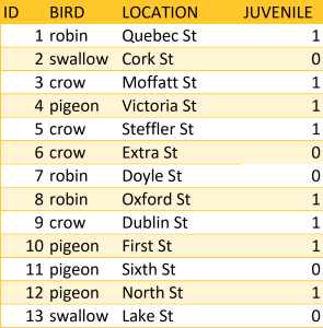
 You may obtain a dataset with variables defined as strings (these may include numbers, letters, or symbols). Numeric functions, such as addition or subtraction, cannot be used on string variables, so in order to run any sort of quantitative data analysis, you’ll need to convert values in string format to numeric values. Looking at the table of bird sightings (Table 7), there is a column indicating whether the bird is a juvenile. To run quantitative data analysis, you’ll need to convert string values of “no” to the numeric value of 0 and string values of “yes” to the numeric value of 1. Leave the original JUVENILE column for reference and create another column with the numeric values. The original column is used to verify the transformation of the new column and is deleted once the transformation is confirmed to be correct. For this example, the new column, JUVENILE _NUM, contains the numeric values of the string values from the JUVENILE column (Tip 06 Exercise).
Numbers can be formatted in different ways, especially with finance data. For example, negative values can be represented with a hyphen or placed inside parentheses or are sometimes highlighted in red. Not all these negative values will be correctly read by a computer, particularly the colour option. When cleaning data, choose and apply a clear and consistent approach to formatting all negative values. A common choice is to use a negative sign.
Tip 06 Exercise: Numbers and Signs
Create a new column named JUVENILE_NUM as part of Table 7. Record a value of 0 in the JUVENILE_NUM column when “no” appears in the JUVENILE column. Record a value of 1 in the JUVENILE_NUM column when “yes” appears in the JUVENILE column.
View Solutions for answers.
Tip 7: Dates and Time
 There are many ways to format dates in a dataset. Sometimes dates are formatted as strings. If date data are needed for analysis, then at a minimum, change the field type from “string” to “date” so dates are recognized in the analysis tool of choice. With time values, you will need to select a convention and use it throughout the dataset. For example, you can choose to use either the 12- or 24-hour clock to define time in a dataset, but whichever you choose, you should be consistent throughout. You may also need to change the format to ensure that all dates and times are formatted in the same way.
Tip 8: Merge and Split Columns
 After closer inspection of the newly acquired dataset, there may be a chance to either (1) merge two or more columns into one or (2) split one column into two or more. Retain the original columns used to merge or split the columns. Then, use the original columns to verify the transformation of the new column and delete the original once the transformation is confirmed to be correct. For example, you may want to split a column that contains a full name into a first and last name (Table 8). Or you may want to split a column with addresses into street, city, region, and postal code columns. Or the reverse might be true. You may want to merge a first and last name column into a full name column or combine address columns.
Tip 08 Exercise: Merge and Split Columns
In Table 8, split the NAME column into two, for first and last names.
HINT: If using Excel, look for functions to “Combine text from two or more cells into one cell” and “Split text into different columns.”
View Solutions for answers.
Tip 9: Subset Data
 Sometimes data files contain information that is unnecessary for an analysis, so you might want to create a new file containing only variables and/or observations of interest, which will involve selectively removing unwanted columns and/or rows. In this example, the researcher removed the JUVENILE column (Table 9). Or you may need to investigate only certain observations in the file, so you can delete rows in the dataset. In this table, all swallow observations will be deleted. One advantage of this type of cleaning is that programs will run more quickly because the data file is smaller.
Tip o9 Exercise: Subset Data
Create a subset of data in Table 9 to include only observations of juveniles (JUVENILE = 1).
HINT: As always, it is important to keep a copy of your original data.
View Solutions for answers.
Cleaning data is an important activity that focuses on removing inconsistencies and errors, which can impact the accuracy of models. The process of cleaning data also provides an opportunity to look closer at the data to determine whether transformations, recoding, or linking additional data is desired.
4. Enriching Data
Sometimes a dataset may not have all the information needed to answer the research question. This means you need to find other datasets and merge them into the current one. This can be as easy as adding geographical data, such as a postal code or longitude and latitude coordinates; or demographic data, such as income, marital status, education, age, or number of children. Enriching data improves the potential for finding fuller answers to the research question(s) at hand.
It’s also important to verify data quality and consistency within a dataset. Let’s take a closer look at validating data, so that the models provide accurate results.
5. Validating Data
Data validation is vital to ensure data are clean, correct, and useful. Remember the adage by Fuechsel — “garbage in, garbage out.” If the incorrect data are fed into a statistical analysis, then the resulting answers will be incorrect too. A computer program doesn’t have common sense and will process the data it is given, good or bad, and while data validation does take time, it helps maximize the potential for data to respond to the research question(s) at hand. Some common data validation checks include the following:
- Checking column data types and underlying data to make sure they’re what they are supposed to be. For example, a date variable may need to be converted from a string to a date format. If in doubt, convert the value to a string and it can be changed later if need be.
- Examining the scope and accuracy of data by reviewing key aggregate functions, like sum, count, min, max, mean, or other related operations. This is particularly important in the context of actual data analysis. Statistics Canada, for example, will code missing values for age using a number well beyond the scope of a human life in years (e.g. using a number like 999). If these values are inadvertently included in your analysis (due to ‘missing values’ not being explicitly declared) any results involving age will be in error. Calculating and reviewing mean, minimum, maximum, etc. will help identify and avoid such errors.
- Ensuring variables have been standardized. For example, when recording latitude and longitude coordinates for locations in North America, check that the latitude coordinates are positive and the longitude coordinates are negative to avoid mistakenly referring to places on the other side of the planet.
It’s important to validate data to ensure quality and consistency. Once all research questions have been answered, it’s good practice to share the clean data with other researchers where confidentiality and other restrictions allow. Let’s take a closer look at publishing data, so that it can be shared with other researchers.
6. Publishing Data
Having made the effort to clean and validate your data and to investigate whatever research questions you set out to answer, it is a key RDM best practice to ensure your data are available for appropriate use by others. This goal is embodied by the FAIR principles covered elsewhere in this textbook, which aim to make data Findable, Accessible, Interoperable, and Reusable. Publishing data helps achieve this goal.
While the best format for collecting, managing, and analyzing data may involve proprietary software, data should be converted to nonproprietary formats for publication. Generally, this will involve plain text. For simple spreadsheets, converting data to CSV (comma separated values) may be best, while more complex data structures may be best suited to XML. This will guard against proprietary formats that quickly become obsolete and will ensure data are more universally available to other researchers going forward. This is discussed more in chapter 9, “A Glimpse Into the Fascinating World of File Formats and Metadata.”
If human subject data or other private information is involved, you may need to consider anonymizing or de-identifying the data (which is covered in chapter 13, “Sensitive Data”). Keep in mind that removing explicit reference to individuals may not be enough to ensure they cannot be identified. If it’s impossible to guard against unwanted disclosure of private information, you may need to publish a subset of the data that is safe for public exposure.
For other researchers to make use of the data, include documentation and metadata, including documentation at the levels of the project, data files, and data elements. A data dictionary outlines the names, definitions, and attributes of the elements in a dataset and is discussed more in chapter 10. You should also document any scripts or methods that have been developed for analyzing the data.
Data Cleaning Software
OpenRefine (https://openrefine.org/) is a powerful data manipulation tool that cleans, reshapes, and batch edits messy and unstructured data. It works best with data in simple tabular formats, like spreadsheets (CSV), or tab-separated values files (TSV), to name a few. OpenRefine is as easy to use as an Excel spreadsheet and has powerful database functions, like Microsoft Access. It is a desktop application that uses a browser as a graphical interface. All data processing is done locally on your computer. When using OpenRefine to clean and transform data, users can facet, cluster, edit cells, reconcile, and use extended web services to convert a dataset to a more structured format. There’s no cost to use this open source software and the source code is freely available, along with modifications by others. There are other tools available for data cleaning, but these are often costly, and OpenRefine is extensively used in the RDM field. If you choose to use other data cleaning software, always check to see if your data remain on your computer or are sent elsewhere for processing.
Exercise: Clean and Prepare Data for Analysis using OpenRefine
Go to the “Cleaning Data with OpenRefine” tutorial and download the Powerhouse museum dataset, consisting of detailed metadata on the collection objects, including title, description, several categories the item belongs to, provenance information, and a persistent link to the object on the museum website. You will step through several data cleaning tasks.
Conclusion
We have covered the six core data cleaning and preparation activities of discovering, structuring, cleaning, enriching, validating, and publishing. By applying these important RDM practices, your data will be complete, documented, and accessible to you and future researchers. You will satisfy grant, journal, and/or funder requirements, raise your profile as a researcher, and meet the growing data-sharing expectations of the research community. RDM practices like data cleaning are crucial to ensure accurate and high-quality research.
Key Takeaways
- Data cleaning is an important task that improves the accuracy and quality of data ahead of data analysis.
- Six core data cleaning tasks are discovering, structuring, cleaning, enriching, validating, and publishing.
- OpenRefine is a powerful data manipulation tool that cleans, reshapes, and batch edits messy and unstructured data.
Reference List
Behrens, J. T. (1997). Principles and procedures of exploratory data analysis. Psychological Methods, 2(2), 131.
Lidwell, W., Holden, K., & Butler, J. (2010). Universal principles of design, revised and updated: 125 ways to enhance usability, influence perception, increase appeal, make better design decisions, and teach through design. Rockport Publishers.
a term that describes all the activities that researchers perform to structure, organize, and maintain research data before, during, and after the research process.
the process of employing six core activities: discovering, structuring, cleaning, enriching, validating, and publishing data.
a process used to explore, analyze, and summarize datasets through quantitative and graphical methods. EDA makes it easier to find patterns and discover irregularities and inconsistencies in the dataset.
guiding principles to ensure that machines and humans can easily discover, access, interoperate, and properly reuse information. They ensure that information is findable, accessible, interoperable, and reusable.
interoperability requires that data and metadata use formalized, accessible, and widely used formats. For example, when saving tabular data, it is recommended to use a .csv file over a proprietary file such as .xlsx (Excel). A .csv file can be opened and read by more programs than an .xlsx file.
a delimited text file that uses a comma to separate values within a data record.
data about data; data that define and describe the characteristics of other data.
an open source data manipulation tool that cleans, reshapes, and batch edits messy and unstructured data.
a format in which information are entered into a table in rows and columns.
a delimited text file that uses a comma to separate values within a data record.
when software is open source, users are permitted to inspect, use, modify, improve, and redistribute the underlying code. Many programmers use the MIT License when publishing their code, which includes the requirement that all subsequent iterations of the software include the MIT license as well.
