Appendix 3: Chapter 10 Exercises

Edited by Kristi Thompson; Elizabeth Hill; Emily Carlisle-Johnston; Danielle Dennie; Émilie Fortin

Appendix 3: Chapter 10 Exercises

Introduction

The purpose of this exercise is to demonstrate the relationship between open data, electronic lab notebooks (ELN), and software containers in reproducible research. You will interact with code in a published ELN, which is hosted in GitHub and made interoperable by myBinder. Many of the fundamentals you learned in chapter 10 will be illustrated here.

This exercise has both an introductory and an advanced activity. In the introductory activity, you will explore the code on GitHub and examine a static version of an ELN. In the advanced activity, you will launch a software container in an interface called Binder. The container hosts an electronic lab notebook that queries an open dataset. You can interact with it online without altering the original copy. The online container allows you to run the code without installing any programs on your computer. The advanced activity requires a higher knowledge of coding, or simply the perseverance to keep trying. The software container doesn’t always load on the first try, and the code won’t work unless it is perfectly entered. This exercise is meant to show benefits and complexity of reproducible research. Don’t be afraid to Google terms that you don’t understand. Additionally, ChatGPT is really good at explaining code and how it functions.

At the very end of the exercise there is a reflection question. You can answer this question even if you haven’t done the advanced activity.

Part 1 (Introductory): Explore the Data and the Code Repository

The Programme for International Student Assessment (PISA) is an international initiative that measures the educational attainment of 15-year-old students. The openly available dataset is available to researchers for their own analyses. This activity uses an analysis of the PISA dataset conducted by Klajnerok (2021), which was published to GitHub using a Jupyter Notebook.

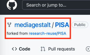
The repository was forked into a new GitHub repository so we could use it for this activity: https://github.com/mediagestalt/PISA. In GitHub, a fork is a copy of a dataset that retains a link to the original creators (“Fork a repo,” n.d.). In the following image, you can see the fork symbol and a link to the dataset that precedes this one. These linkages are important as they show the provenance of the dataset.

A screenshot of a forked repository in GitHub. The name of the new reads mediagestalty/PISA. The screenshot says that the new repository is forked from research-reuse/PISA. Beside the name of the repository, there is a tag that says it is a public repository. — **Figure 1.** *Forked repository.*

QUESTION 1: What is the name of the repository from which this code originated?

Answer: The original creator of the code is https://github.com/mklajnerok/PISA. For this project, the code and data were reused by https://github.com/research-reuse/PISA and placed into a software container called Binder. This assignment is a fork of https://github.com/research-reuse/PISA, and adapted for this textbook. The original dataset was published by PISA.

You can navigate GitHub as you would any nested file directory. In the image that follows, you will see a screenshot of GitHub. The filenames are in the left column, the middle column shows the comment that was left to describe the last changes to the file, and the right column shows the last time the file was edited. You can also see the last person that contributed to the code repository at the top left of the table and the versioning information at the top right of the table, shown in the following image as “83 commits.”

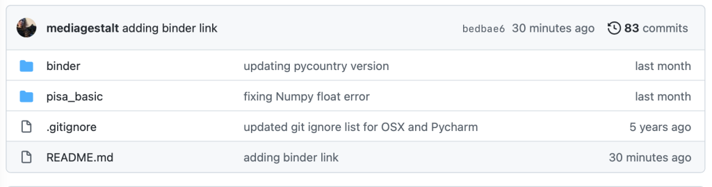
GitHub Folders

For the next question, find the following files in the repository. You will find the files in different folders, so don’t be afraid to look around.

requirements.txt
pisa_project_part1.ipynb

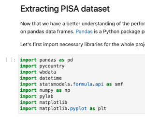
Click on the title of a file to view it. Then, scroll down to view the content of each file. You are looking for a list of dependencies, which are the software packages required to run the code in the notebook. In the pisa_project_part1.ipynb file, you will find the list under the heading “Extracting PISA dataset,” as shown in the following image.

A screenshot of files of the pisa_project_part1.ipynb file. At the top, there is a heading that reads, “Extracting PISA dataset.” Below that is some text that is not all shown in the screenshot, but reads, “Now that we have a better understanding of the perfor… on pandas data frames. Pandas is a Python package p… Let’s first import necessary libraries for the whole proj…”Below that is the list of dependences that reads: Import pandas as pd Import pycountry Import wbdata Import datetime Import statsmodels.formula.api as smf Import numpy as np Import pylab Import matplotlib Import matplotlib.pyplot as plt — **Figure 3.** *Notebook dependencies.*

QUESTION 2: Compare the dependencies listed in requirements.txt with those listed in the pisa_project_part1.ipynb notebook. What is different?

Answer: The requirements.txt file includes the version numbers of the dependencies; the notebook file simply lists the names. Versioning information for dependencies is very important because unknown changes to dependencies may prevent the code from working properly, or at all. This is a scenario where updating to the newest version of a program is not always preferred. Curating code for reuse is essentially freezing the code ‘in time,’ so that it runs exactly as it did when it was created.

The file names and directories show the importance of relative file paths. In the Git directory, find the location of the following .csv files and match them to where they are named in the notebook file.

pisa_math_2003_2015.csv
pisa_read_2000_2015.csv
pisa_science_2006_2015.csv. Hint: the files are listed in the second code cell below the dependencies.

Part 2 (Advanced): Run and Alter the Code

It is time to explore the software container. Since the original researcher wrote the code in a Jupyter Notebook (a commonly-used ELN), it is possible to ‘containerize’ the code and the data so that it can be run by other users.

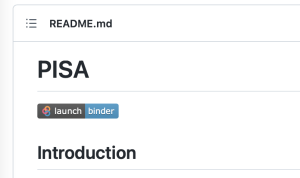
Return to the main page of the GitHub repository, also known as the README file. Then, click on the launch binder button, shown in the following image.

A screenshot of the README file. It says README.md at the top. Below that is a header titled, “PISA.” Followed by a gray and blue icon that says, “launch binder.” — **Figure 4.** *Launch binder.*

Depending on your computer and your internet speed, the software container may take several minutes to load. If it takes too long, just close the page and try launching again from the GitHub Binder link. You can see the Binder loading screen in the following image.

The binder loading screen, containing large text that reads “binder.” Beneath that is text that reads, “Starting repository” mediagestalt/PISA/HEAD” and “New to Binder? Check out the Binder Documentation for more information.” — **Figure 5.** *Launch binder 2.*

When the notebook loads, scroll down and explore the page. The live notebook looks exactly like the notebook file you viewed in the GitHub repository.

As you examine the notebook, you will see narrative text interspersed with blocks of code inside defined cells. There is additional commentary inside the code cells. This is what literate programming looks like.

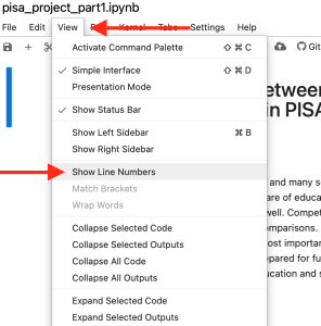
To make the next part of the activity easier, turn on the line numbers in the file. This will show a number on each line of the code block, making it easier to identify specific lines of code. The location of this command is shown in the next image. You won’t see an immediate change to the page, as this is just a setting change.

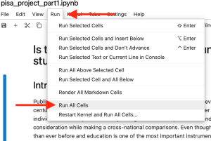
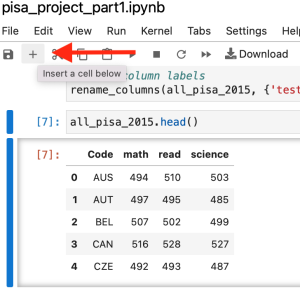
A screenshot of the Show Line Numbers command in the file. A red arrow is pointing to the “View” command, which is the third command from the left in the file task bar. The View command window is open, and another red arrow is pointing to the “Show Line Numbers” command, which is the 7th command from the top. — **Figure 6.** *Toggle line numbers.*

Now it is time to run the code. To start, you must run all of the code cells. The location of this command is shown in the following image. As you scroll down the page, you will begin to see new content below some of the code blocks. These are the results of the analysis for which the code was written. There may be text, tables, or visualizations.

A screenshot of the Run All Cells command in the file. A red arrow is pointing to the “Run” command, which is the fourth command from the left in the file task bar. The Run command window is open, and another red arrow is pointing to the “Run All Cells” command, which is the 8th command from the top. — **Figure 7.** *Run all of the cells.*

You will also see a number in square brackets in the left margin beside each block of code. Start at the beginning of the page and read down until you reach cell number 6. Don’t worry if you don’t understand the code. Pay more attention to the textual descriptions, and the comments inside the cells. You can identify a comment because it will be preceded by a [#] or [“””] symbol. Read the narrative descriptions until you reach cell #6. It is shown in the following image.

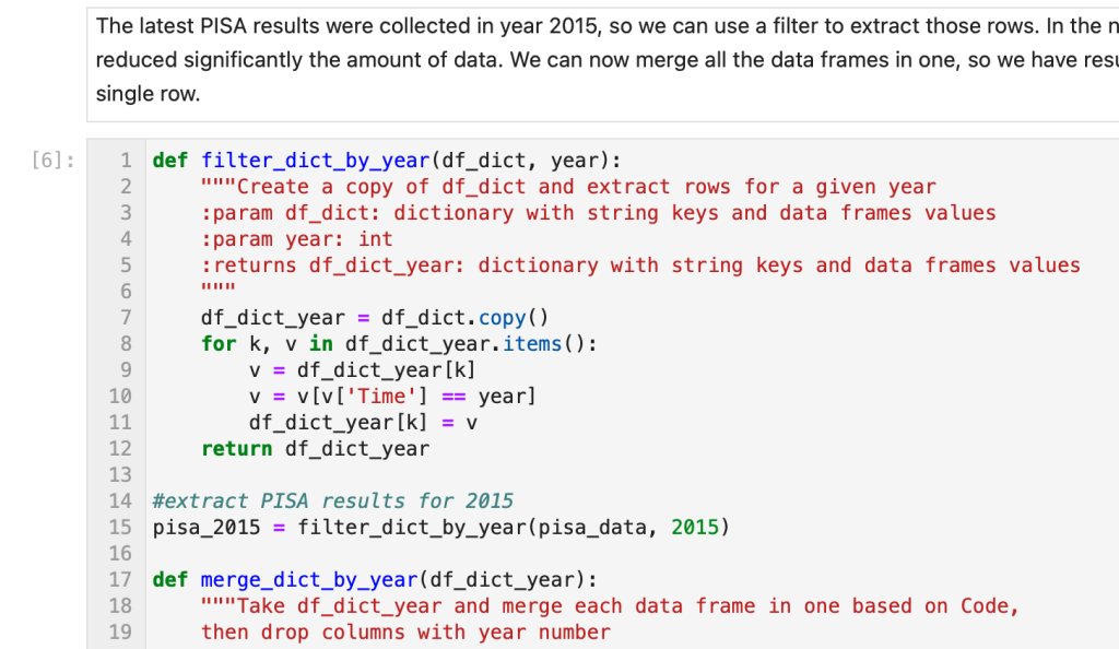
A screenshot of the code in cell 6. The screenshot shows lines 1 through 19. Line 14 reads, “#extract PISA results for 2015.” — **Figure 8.** *Cell 6.*

QUESTION 3: What does the comment on line 14 of cell 6 say?

Answer: #extract PISA results for 2015. Hint: If you didn’t find it, use the ‘Find’ feature in your browser to search for the phrase. Then, you’ll see the line and cell number.

The PISA dataset in this project has data going back to 2000. We can load more data by altering the code. For the next part of this activity, you will need to add new code to the ELN and re-run the code block. To get the additional lines of code, go to this code snippet (called a Gist) in GitHub. It is an edited version of cell 6 in the notebook.

Line 14 in the Gist and line 14 in code block 6 in the notebook are the same. The ‘#’ before the text means that the line is a comment, not live code. Line 15 is where the code starts. In this Gist, there are extra lines of code below line 15 that don’t appear in the notebook. Copy the code from lines 16 and 17 and paste them in the notebook. Make sure the notebook matches lines 14-17 in the Gist.

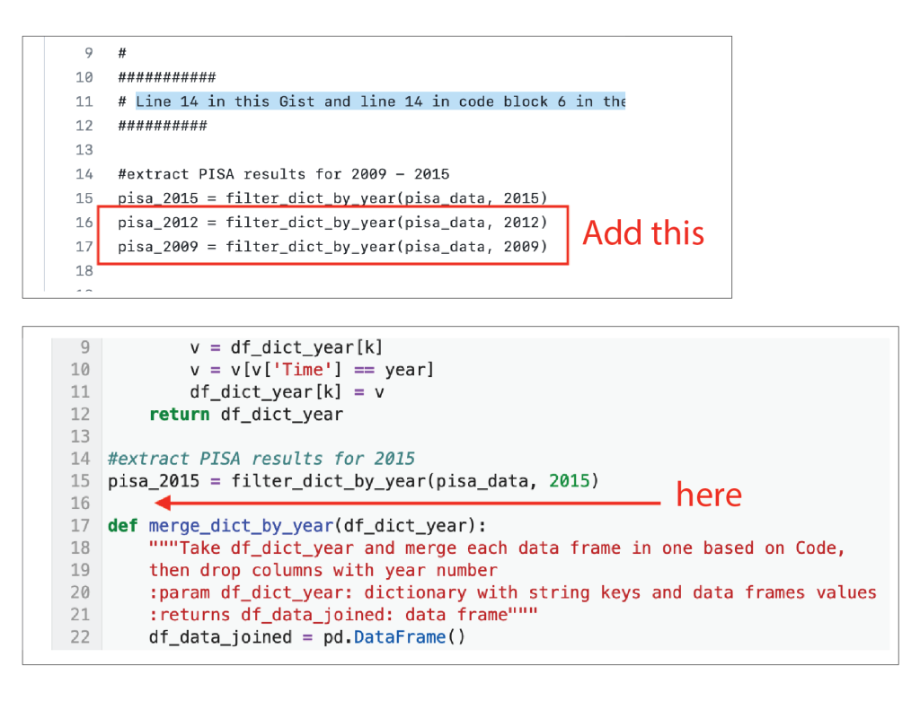
A small textbox, showing a screenshot of code in lines 9 through 18. There is a red box around the code in lines 16 and 17, with instruction in red text that reads, “Add this.” The code in line 16 reads, “pisa_2012 = filder_dict_by_year(pisa_data, 2012). The code in line 17 reads, “pisa_2009 = filter_dict_by_year(pisa_data, 2009)”.Below the smaller textbox is a larger one, also showing code. This screenshot shows lines 9 through 22. In line 16, there is a red arrow and red text that reads “here.” — **Figure 9.** *Gist code*.

This code is calling on the PISA dataset. Before you added the extra lines, the data from PISA was from 2015 only. Adding the two extra lines of code imports additional years of data from PISA (2012 and 2009). If you want to experiment more, you can add additional lines with different years. Just be sure to follow the format exactly as you see it.

Adding just these lines isn’t enough. You’ll need to follow the same process for lines #31 and #40. This code and more instructions can also be found in the Gist. Note that the line numbers in the notebook will change when you add additional code.

Once you’ve added the extra parameters to the notebook, re-run cell 6 in the notebook by clicking in the cell and pressing shift + return. If there are any errors, check your code for typos and try again. You can also use the Run > Run Selected Cells menu command.

From here on, the cell numbers in the notebook will change depending on how many times you run the code within that cell.

Next, keep your cursor in the cell you just edited, and then insert a new cell for each of the additional years you’ve added.

A screenshot showing how to a a new cell. In the second toolbar from the top, there is an icon in the shape of a plus sign (located just to the right of the “save” icon). Clicking this icon will insert a cell below. — **Figure 10.** *Add new cells.*

Type the additional variable names for the years you’ve added into the new cells and press shift + return to run each one.

For example: all_pisa_2012.head() all_pisa_2009.head()

If there are errors, check for typos and try again.

See how many other cells you can get to work! Both with the existing variables, and the new variables you’ve created.

If you make a mistake and break the code beyond repair, you can check the source file to copy and paste the original code. You can also reload the file completely with File > Reload Notebook from Disk in the notebook top menu.

Reflective Questions

Based on what you’ve learned in chapter 10 and your exploration of the software container, what changes would you make to the structure of the file directory to improve the organization? Have the data and software been adequately documented? Work through the Reproducibility Framework (Khair, Sawchuk, and Zhang, 2019) to help with your assessment.
1. Is the provenance of these data clear to you? Explain.
2. What features of this dataset have enabled its reproducibility? What would you improve?

Reference List

Fork a repo. (n.d.). GitHub docs. https://docs.github.com/en/get-started/quickstart/fork-a-repo

Klajnerok, M. (2021). Is there a relationship between countries’ wealth or spending on schooling and its students’ performance in PISA? Medium. https://towardsdatascience.com/is-there-a-relationship-between-countries-wealth-or-spending-on-schooling-and-its-students-a9feb669be8c

Khair, S., Sawchuk, S., Zhang, Q. (2019). Reproducibility Framework. https://docs.google.com/document/d/1E0c5-DDVo2MMoF2rPOiH2brIZyC_3YZZrcgp0x6VCPs/edit

License

Icon for the Creative Commons Attribution-NonCommercial 4.0 International License

Research Data Management in the Canadian Context Copyright © 2023 by Edited by Kristi Thompson; Elizabeth Hill; Emily Carlisle-Johnston; Danielle Dennie; and Émilie Fortin is licensed under a Creative Commons Attribution-NonCommercial 4.0 International License, except where otherwise noted.