Polynomial and Rational Functions

OER Lab

9 Polynomial and Rational Functions

Chapter 9 Topics

9.1 Quadratic Functions

9.2 Polynomial Functions

9.3 Rational Functions

9.1 Quadratic Functions

In this section, we will explore the quadratic functions, a type of polynomial function. Quadratics commonly arise from problems involving areas, as well as revenue and profit, providing some interesting applications.

Example 9.1A: Understanding Quadratic Functions

A backyard farmer wants to enclose a rectangular space for a new garden. She has purchased 80 feet of wire fencing to enclose 3 sides, and will put the 4th side against the backyard fence. Find a formula for the area enclosed by the fence if the sides of fencing perpendicular to the existing fence have length L.

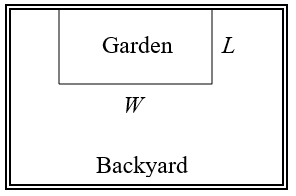
In a scenario like this involving geometry, it is often helpful to draw a picture. It might also be helpful to introduce a temporary variable, W, to represent the side of fencing parallel to the 4th side or backyard fence.

Since we know we only have 80 feet of fence available, we know that , or more simply, . This allows us to represent the width, W, in terms of L:

Now we are ready to write an equation for the area the fence encloses. We know the area of a rectangle is length multiplied by width, so

This formula represents the area of the fence in terms of the variable length L.

Short run Behavior: Vertex

We now explore the interesting features of the graphs of quadratics. In addition to intercepts, quadratics have an interesting feature where they change direction, called the vertex.

The standard form for a quadratic is $f(x) = a{x^2} + bx + c$ , but you will often see them written in the form $f(x) = a{(x - h)^2} + k$ . To see why, consider this example.

Example 9.1B: Vertex of the Quadratic

Sketch a graph of $g(x) = \frac{1}{2}{(x + 2)^2} - 3$

We can create a table of values, which we can use to plot several points and connect them with a smooth curve.

x	g(x)
-5	1.5
-4	-1
-3	-2.5
-2	-3
-1	-2.5
0	-1
1	1.5

Notice that the turning point of the graph, where it changes from decreasing to increasing, is at the point (-2, -3). We call this point the vertex of the quadratic. Notice that $g(x) = \frac{1}{2}{(x + 2)^2} - 3$ can also be written as $g(x) = \frac{1}{2}{\left( {x - \left( { - 2} \right)} \right)^2} - 3$ . Comparing that to the form $f(x) = a{(x - h)^2} + k$ , you can see that the vertex of the graph, (-2, -3), corresponds with the point (h, k).

Forms of Quadratic Functions

The standard form of a quadratic function is $f(x) = a{x^2} + bx + c$

The vertex form of a quadratic function is $f(x) = a{(x - h)^2} + k$

The vertex of the quadratic function is located at (h, k), where h and k are the numbers in the vertex form of the function.

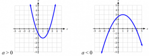
When a > 0, the graph of the quadratic will open upwards.

When a < 0, the graph of the quadratic will open downwards.

Give It Some Thought

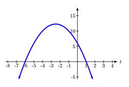
A coordinate grid has been superimposed over the quadratic path of a basketball[1]. Find an equation for the path of the ball. Does he make the basket?

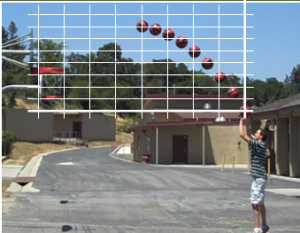
[1] From http://blog.mrmeyer.com/?p=4778, © Dan Meyer, CC-BY

Example 9.1C: Standard Polynomial Function

Write $g(x) = \frac{1}{2}{(x + 2)^2} - 3$ in standard form.

To write this in standard polynomial form, we could expand the formula and simplify terms:

$\begin{array}{l} g(x) = \frac{1}{2}{(x + 2)^2} - 3\\ g(x) = \frac{1}{2}(x + 2)(x + 2) - 3\\ g(x) = \frac{1}{2}({x^2} + 4x + 4) - 3\\ g(x) = \frac{1}{2}{x^2} + 2x + 2 - 3\\ g(x) = \frac{1}{2}{x^2} + 2x - 1 </div> \end{array}$

In the previous example, we saw that it is possible to rewrite a quadratic function given in vertex form and rewrite it in standard form by expanding the formula. It would be useful to reverse this process, since the transformation form reveals the vertex.

Expanding out the general transformation form of a quadratic gives:

$\begin{array}{l} f(x) = a{(x - h)^2} + k = a(x - h)(x - h) + k\\ f(x) = a({x^2} - 2xh + {h^2}) + k = a{x^2} - 2ahx + a{h^2} + k \end{array}$

This should be equal to the standard form of the quadratic:

$a{x^2} - 2ahx + a{h^2} + k = a{x^2} + bx + c$

The second degree terms are already equal. For the linear terms to be equal, the coefficients must be equal:

$- 2ah = b$ , so $h = - \frac{b}{{2a}}$

This provides us a method to determine the horizontal shift of the quadratic from the standard form. We could likewise set the constant terms equal to find:

$a{h^2} + k = c$ , so $k = c - a{h^2} = c - a{\left( { - \frac{b}{{2a}}} \right)^2} = c - a\frac{{{b^2}}}{{4{a^2}}} = c - \frac{{{b^2}}}{{4a}}$

In practice, though, it is usually easier to remember that k is the output value of the function when the input is h, so $k = f(h)$ .

Finding the Vertex of a Quadratic

For a quadratic given in standard form, the vertex (h, k) is located at:

$h = - \frac{b}{{2a}}$ , $k = f(h) = f\left( {\frac{{ - b}}{{2a}}} \right)$

Example 4

Find the vertex of the quadratic $f(x) = 2{x^2} - 6x + 7$ . Rewrite the quadratic into vertex form.

The horizontal coordinate of the vertex will be at $h = - \frac{b}{{2a}} = - \frac{{ - 6}}{{2(2)}} = \frac{6}{4} = \frac{3}{2}$

The vertical coordinate of the vertex will be at $f\left( {\frac{3}{2}} \right) = 2{\left( {\frac{3}{2}} \right)^2} - 6\left( {\frac{3}{2}} \right) + 7 = \frac{5}{2}$

Rewriting into vertex form, the value of a will remain the same as in the original quadratic.

$f(x) = 2{\left( {x - \frac{3}{2}} \right)^2} + \frac{5}{2}$

Give It Some Thought

2. Given the equation g(x)=13+x²=6x write the equation in standard form and then in vertex form.

In addition to enabling us to more easily graph a quadratic written in standard form, finding the vertex serves another important purpose – it allows us to determine the maximum or minimum value of the function, depending on which way the graph opens.

Example 9.1D: Finding the Vertex

Returning to our backyard farmer from the beginning of the section, what dimensions should she make her garden to maximize the enclosed area?

Earlier we determined the area she could enclose with 80 feet of fencing on three sides was given by the equation $A(L) = 80L - 2{L^2}$ . Notice that quadratic has been vertically reflected, since the coefficient on the squared term is negative, so the graph will open downwards, and the vertex will be a maximum value for the area.

In finding the vertex, we take care since the equation is not written in standard polynomial form with decreasing powers. But we know that a is the coefficient on the squared term, so a = -2, b = 80, and c = 0.

Finding the vertex:

$h = - \frac{{80}}{{2( - 2)}} = 20$ , $k = A(20) = 80(20) - 2{(20)^2} = 800$

The maximum value of the function is an area of 800 square feet, which occurs when L = 20 feet. When the shorter sides are 20 feet, that leaves 40 feet of fencing for the longer side. To maximize the area, she should enclose the garden so the two shorter sides have length 20 feet, and the longer side parallel to the existing fence has length 40 feet.

Example 9.1E: Maximum Revenue

A local newspaper currently has 84,000 subscribers, at a quarterly charge of $30. Market research has suggested that if they raised the price to $32, they would lose 5,000 subscribers. Assuming that subscriptions are linearly related to the price, what price should the newspaper charge for a quarterly subscription to maximize their revenue?

Revenue is the amount of money a company brings in. In this case, the revenue can be found by multiplying the charge per subscription times the number of subscribers. We can introduce variables, C for charge per subscription and S for the number subscribers, giving us the equation:

Revenue = CS

Since the number of subscribers changes with the price, we need to find a relationship between the variables. We know that currently S = 84,000 and C = 30, and that if they raise the price to $32 they would lose 5,000 subscribers, giving a second pair of values, C = 32 and S = 79,000. From this we can find a linear equation relating the two quantities. Treating C as the input and S as the output, the equation will have form $S = mC + b$ . The slope will be $m = \frac{{79,000 - 84,000}}{{32 - 30}} = \frac{{ - 5,000}}{2} = - 2,500$

This tells us the paper will lose 2,500 subscribers for each dollar they raise the price. We can then solve for the vertical intercept

$S = - 2500C + b$

Plug in the point S = 84,000 and C = 30

$84,000 = - 2500(30) + b$

Solve for b:

$b = 159,000$

This gives us the linear equation $S = - 2,500C + 159,000$ relating cost and subscribers. We now return to our revenue equation.

Substituting the equation for S from above:

Revenue = CS

Revenue = C(-2,500C+159,000)

Expanding:

Revenue = -2,500C²+159,000C

We now have a quadratic equation for revenue as a function of the subscription charge. To find the price that will maximize revenue for the newspaper, we can find the vertex:

$h = - \frac{{159,000}}{{2( - 2,500)}} = 31.8$

The model tells us that the maximum revenue will occur if the newspaper charges $31.80 for a subscription. To find what the maximum revenue is, we can evaluate the revenue equation:

Maximum Revenue = -2,500(31.8)²+159,000(31.8)=2,528,100

Notice that the equation S= -2,500C+159,000 we found in the last example is essentially a demand function – a relationship between the price (C) and the demand (S). This is a common type of economic application.

Maximizing Revenue or Profit

To solve a problem involving maximizing revenue or profit given data on demand at different price levels,

1. Use the data provided to create a demand equation relating price and quantity demanded. This will usually be a linear function.

2. Create a Revenue equation. Start with Revenue = price times quantity, then substitute the demand equation to create a revenue equation just in terms of quantity.

3. If the problem is to maximize profit, create a Profit equation. Profit = revenue minus cost.

4. Find the vertex of the Revenue or Profit function to find the quantity that maximizes revenue or profit.

5. If needed, use that quantity with the demand function to find the price that maximizes revenue or profit.

Example 9.1F: Maximum and Total Profit

A company is planning to sell a new smart fitness device. Developing the product will cost $700,000, and each product will cost $30 to manufacture. Market research suggests that if they sell the device for $100, they will be able to sell 30,000 items. For each $10 they lower the price, they estimate they will sell 5,000 more items. Assuming quantity demanded is linearly related to price, determine the price that will maximize profit

Let p be the price per item, and q be the quantity the company can sell. We start by creating a linear demand function, of the form p = mq + b.

If they sell the device for $100, they will be able to sell 30,000 items, giving the point (30000, 100).

We are told that for each $10 they lower the price, they estimate they will sell 5,000 more items. We can either directly interpret this as a slope, or use it to create a second point. Lowering the price to $90 would raise the quantity sold to 35,000, giving a second point (35000, 90).

Finding the slope:

The demand equation will look like p = – 0.002q + b . Substituting in (30000, 10) to solve for b:

100 = – 0.002 (30000) + b

100 = – 60 + b

b = 160

We now have our demand function: p = – 0.002q + 160 .

Now we construct our revenue function, using our demand curve

R = pq

Substituting in the demand function for p

R = (- 0.002q + 160)q = – 0.002q² + 160q)

Now looking at costs, we know the fixed costs are $700,000, and the per-item costs are $30, leading to the cost equation

C = 700,00 + 30q

Finally we can construct the profit equation:

Profit = Revenue – Cost

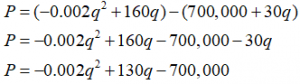
Now to find the maximum we find the vertex of the quadratic:

To find the price that will produce a demand of 32,500 items, we use the demand function:

P = – 0.002(32500) + 160 = 95

To maximize profit, the company should price the device at $95. At that price they should expect to sell 35,000 items, with a total profit of:

P = – 0.002(32500)²+ 130(32500) – 70,000 = $1,412,500

Short run Behavior: Intercepts

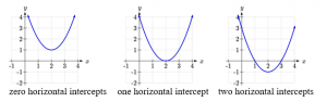
As with any function, we can find the vertical intercepts of a quadratic by evaluating the function at an input of zero, and we can find the horizontal intercepts by solving for when the output will be zero. Notice that depending upon the location of the graph, we might have zero, one, or two horizontal intercepts.

Example 9.1G: Vertical and Horizontal Intercepts

Find the vertical and horizontal intercepts of the quadratic $f(x) = 3{x^2} + 5x - 2$

We can find the vertical intercept by evaluating the function at an input of zero:

$f(0) = 3{(0)^2} + 5(0) - 2 = - 2$ Vertical intercept at (0,-2)

For the horizontal intercepts, we solve for when the output will be zero $0 = 3{x^2} + 5x - 2$

In this case, the quadratic can be factored easily, providing the simplest method for solution

0= (3x-1)(x+2)

$0 = 3x - 1\\ x = \frac{1}{3}<span style="font-size: 1em">$ or

$\0 = x + 2\\ x = - 2$

Horizontal intercepts at and (-2,0)

Notice that in the standard form of a quadratic, the constant term c reveals the vertical intercept of the graph.

For quadratics that can’t be factored, we need another tecnique. Based on our previous work we showed that any quadratic in standard form can be written into vertex form as:

$f(x) = a{\left( {x + \frac{b}{{2a}}} \right)^2} + c - \frac{{{b^2}}}{{4a}}$

Solving for the horizontal intercepts using this general equation gives:

$0 = a{\left( {x + \frac{b}{{2a}}} \right)^2} + c - \frac{{{b^2}}}{{4a}}$ start to solve for x by moving the constants to the other side divide both sides by a

$\frac{{{b^2}}}{{4{a^2}}} - \frac{c}{a} = {\left( {x + \frac{b}{{2a}}} \right)^2}$ find a common denominator to combine fractions

$\frac{{{b^2}}}{{4{a^2}}} - \frac{{4ac}}{{4{a^2}}} = {\left( {x + \frac{b}{{2a}}} \right)^2}$ combine the fractions on the left side of the equation

$\frac{{{b^2} - 4ac}}{{4{a^2}}} = {\left( {x + \frac{b}{{2a}}} \right)^2}$ take the square root of both sides

$\pm \sqrt {\frac{{{b^2} - 4ac}}{{4{a^2}}}} = x + \frac{b}{{2a}}$ subtract b/2a from both sides

$- \frac{b}{{2a}} \pm \frac{{\sqrt {{b^2} - 4ac} }}{{2a}} = x$ combining the fractions

$x = \frac{{ - b \pm \sqrt {{b^2} - 4ac} }}{{2a}}$ Notice that this can yield two different answers for x

Quadratic Formula

For a quadratic function given in standard form , the quadratic formula gives the horizontal intercepts of the graph of this function.

$x = \frac{{ - b \pm \sqrt {{b^2} - 4ac} }}{{2a}}$

Example 1.9H: Equilibrim

The supply for a certain product can be modeled by p=3q2 and the demand can be modeled by p=1620=2q2, where p is the price in dollars, and q is the quantity in thousands of items. Find the equilibrium price and quantity.

Recall that the equilibrium price and quantity is found by finding where the supply and demand curve intersect. We can find that by setting the equations equal:

$3{q^2} = 1620 - 2{q^2}$

Add 2q² to both sides

5q²= 1620 Divide by 5 on both sides

q²= 324 Take the square root of both sides

$q = \pm \sqrt {324} = \pm 18$

Since it doesn’t make sense to talk about negative quantities, the equilibrium quantity is q = 18. To find the equilibrium price, we evaluate either function at the equilibrium quantity.

p= 3(18)²= 972

The equilibrium is 18 thousand items, at a price of $972.

Give It Some Thought

3. For these two equations determine if the vertex will be a maximum value or a minimum value.

a. $g(x) = - 8x + {x^2} + 7$

b. $g(x) = - 3{(3 - x)^2} + 2$

Give It Some Thought Answers

1. The path passes through the origin with vertex at (-4, 7). . To make the shot, h(-7.5) would need to be about 4. h(-7.5) = 1.64; he doesn’t make it.

2. g(x) = x2 + 6x + 13 in Standard form; in Transformation form g(x) = (x – 3)2 + 4

3. a. Vertex is a minimum value

b. Vertex is a maximum value

9.2 Polynomial Functions

In the previous section we explored the short run behavior of quadratics, a special case of polynomials. In this section we will explore the behavior of polynomials in general. The basic building blocks of polynomials are power functions.

Power Functions

A power function is a function that can be represented in the form $f(x) = {x^p}$ %

Where the base is a variable and the exponent, p, is a number.

Characteristics of Power Functions

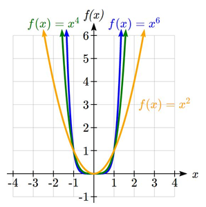
Shown to the right are the graphs of f(x) = x², f(X) =x⁴, and f(X) = x⁶, all even whole number powers. Notice that all these graphs have a fairly similar shape, very similar to a quadratic, but as the power increases the graphs flatten somewhat near the origin, and become steeper away from the origin.

To describe the behavior as numbers become larger and larger, we use the idea of infinity. The symbol for positive infinity is $\infty$ , and $- \infty$ for negative infinity. When we say that “x approaches infinity”, which can be symbolically written as $x \to \infty$ , we are describing a behavior – we are saying that x is getting large in the positive direction.

With the even power function, as the input becomes large in either the positive or negative direction, the output values become very large positive numbers. Equivalently, we could describe this by saying that as x approaches positive or negative infinity, the f(x) values approach positive infinity. In symbolic form, we could write: as $x \to \pm \infty$ , $f(x) \to \infty$ .

Shown here are the graphs of f(x) = x³, f(X) =x⁵, and f(X) = x⁷, all odd whole number powers. Notice all these graphs look similar, but again as the power increases the graphs flatten near the origin and become steeper away from the origin.

For these odd power functions, as x approaches negative infinity, f(x) approaches negative infinity. As x approaches positive infinity, f(x) approaches positive infinity. In symbolic form we write: as $x \to - \infty$ , $f(x) \to - \infty$ and as $x \to \infty$ , $f(x) \to \infty$ .

Long Run Behavior

The behavior of the graph of a function as the input takes on large negative values ( $x \to - \infty$ ) and large positive values ( $x \to \infty$ ) as is referred to as the long run behavior of the function.

Terminology of Polynomial Functions

A polynomial is function that can be written as $f(x) = {a_0} + {a_1}x + {a_2}{x^2} + \cdots + {a_n}{x^n}$

Each of the ai constants are called coefficients and can be positive, negative, or zero, and be whole numbers, decimals, or fractions.

A term of the polynomial is any one piece of the sum, that is any . Each individual term is a transformed power function.

The degree of the polynomial is the highest power of the variable that occurs in the polynomial.

The leading term is the term containing the highest power of the variable: the term with the highest degree.

The leading coefficient is the coefficient of the leading term.

Because of the definition of the “leading” term we often rearrange polynomials so that the powers are descending.

$f(x) = {a_n}{x^n} + ..... + {a_2}{x^2} + {a_1}x + {a_0}^{}$

Example 9.2A: Identifying Degrees, Leading Terms and Leading Coefficient

Identify the degree, leading term, and leading coefficient of these polynomials:

$f(x) = 3 + 2{x^2} - 4{x^3}$

$g(t) = 5{t^5} - 2{t^3} + 7t$

$h(p) = 6p - {p^3} - 2$

For the function f(x), the degree is 3, the highest power on x. The leading term is the term containing that power, -4x³. The leading coefficient is the coefficient of that term, -4.

For g(t), the degree is 5, the leading term is 5t⁵, and the leading coefficient is 5.

For h(p), the degree is 3, the leading term is , so the leading coefficient is -1.

Long Run Behavior of Polynomials

For any polynomial, the long run behavior of the polynomial will match the long run behavior of the leading term.

Example 9.2B: Long Run Behavior and Degree

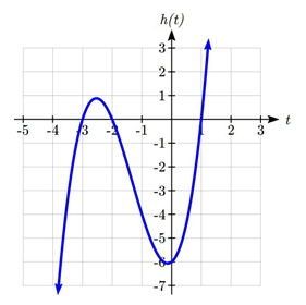
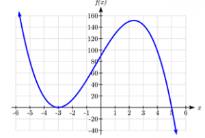
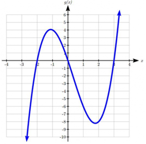
What can we determine about the long run behavior and degree of the equation for the polynomial graphed here?

Since the output grows large and positive as the inputs grow large and positive, we describe the long run behavior symbolically by writing: as $x \to \infty$ , $f(x) \to \infty$ . Similarly, as $x \to - \infty$ , $f(x) \to - \infty$ .

In words, we could say that as x values approach infinity, the function values approach infinity, and as x values approach negative infinity the function values approach negative infinity.

We can tell this graph has the shape of an odd degree power function which has not been reflected, so the degree of the polynomial creating this graph must be odd, and the leading coefficient would be positive.

Short Run Behavior: Intercepts

Characteristics of the graph such as vertical and horizontal intercepts and the places the graph changes direction are part of the short run behavior of the polynomial.

Like with all functions, the vertical intercept is where the graph crosses the vertical axis, and occurs when the input value is zero. Since a polynomial is a function, there can only be one vertical intercept, which occurs at the point (0,a₀). The horizontal intercepts occur at the input values that correspond with an output value of zero. It is possible to have more than one horizontal intercept.

Horizontal intercepts are also called zeros, or roots of the function.

To find horizontal intercepts, we need to solve for when the output will be zero. For general polynomials, this can be a challenging prospect. While quadratics can be solved using the relatively simple quadratic formula, the corresponding formulas for cubic and 4th degree polynomials are not simple enough to remember, and formulas do not exist for general higher-degree polynomials. Consequently, we will limit ourselves to three cases:

1) The polynomial can be factored using known methods: greatest common factor and trinomial factoring.
2) The polynomial is given in factored form.
3) Technology is used to determine the intercepts.

Example 9.2C: Finding Horizontal Intercepts

Find the horizontal intercepts of $f(x) = {x^6} - 3{x^4} + 2{x^2}$ .

We can attempt to factor this polynomial to find solutions for f(x) = 0.

${x^6} - 3{x^4} + 2{x^2} = 0$ Factoring out the greatest common factor

${x^2}\left( {{x^4} - 3{x^2} + 2} \right) = 0$ Factoring the inside as a quadratic in x2

${x^2}\left( {{x^2} - 1} \right)\left( {{x^2} - 2} \right) = 0$ Then break apart to find solutions

$\begin{array}{l} {x^2} = 0\\ x = 0 </div> \end{array}$ or

$\begin{array}{l} \left( {{x^2} - 1} \right) = 0\\ {x^2} = 1\\ x = \pm 1 </div> \end{array}$ or

$\begin{array}{l} \left( {{x^2} - 2} \right) = 0\\ {x^2} = 2\\ x = \pm \sqrt 2 \end{array}$

This gives us 5 horizontal intercepts.

Example 9.2D: Finding Vertical and Horizontal Intercepts

Find the vertical and horizontal intercepts of $g(t) = {(t - 2)^2}(2t + 3)$

The vertical intercept can be found by evaluating g(0).

$g(0) = {(0 - 2)^2}(2(0) + 3) = 12$

The horizontal intercepts can be found by solving g(t) = 0

${(t - 2)^2}(2t + 3) = 0$ Since this is already factored, we can break it apart:

$\begin{array}{l} {(t - 2)^2} = 0\\ t - 2 = 0\\ t = 2 \end{array}$ or

$\begin{array}{l} (2t + 3) = 0\\ t = \frac{{ - 3}}{2} \end{array}$

We can always check our answers are reasonable by graphing the polynomial.

Example 9.2E: Finding Horizontal Intercepts of Non-factorial Polynomial

Find the horizontal intercepts of $h(t) = {t^3} + 4{t^2} + t - 6$

Since this polynomial is not in factored form, has no common factors, and does not appear to be factorable using techniques we know, we can turn to technology to find the intercepts.

Graphing this function, it appears there are horizontal intercepts at t = -3, -2, and 1.

We could check these are correct by plugging in these values for t and verifying that $h( - 3) = h( - 2) = h(1) = 0$ .

Notice that the polynomial in the previous example was degree three, and had three horizontal intercepts and two turning points – places where the graph changes direction. We will now make a general statement without justifying it.

Intercepts and Turning Points of Polynomials

A polynomial of degree n will have:

At most n horizontal intercepts. An odd degree polynomial will always have at least one.

At most n-1 turning points

Give It Some Thought

1. Find the vertical and horizontal intercepts of the function $f(t) = {t^4} - 4{t^2}$ .

Graphical Behavior at Intercepts

If we graph the function $f(x) = (x + 3){(x - 2)^2}{(x + 1)^3}$ , notice that the behavior at each of the horizontal intercepts is different.

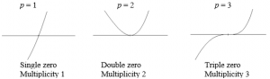
At the horizontal intercept x = -3, coming from the x+3 factor of the polynomial, the graph passes directly through the horizontal intercept. The factor is linear (has a power of 1), so the behavior near the intercept is like that of a line – it passes directly through the intercept. We call this a single zero, since the zero corresponds to a single factor of the function.

At the horizontal intercept x = 2, coming from the (x-2)² factor of the polynomial, the graph touches the axis at the intercept and changes direction. The factor is quadratic (degree 2), so the behavior near the intercept is like that of a quadratic – it bounces off of the horizontal axis at the intercept. Since ${(x - 2)^2} = (x - 2)(x - 2)$ , the factor is repeated twice, so we call this a double zero. We could also say the zero has multiplicity 2.

At the horizontal intercept x = -1, coming from the (x+1)³ factor of the polynomial, the graph passes through the axis at the intercept, but flattens out a bit first. This factor is cubic (degree 3), so the behavior near the intercept is like that of a cubic, with the same “S” type shape near the intercept that the toolkit has. We call this a triple zero. We could also say the zero has multiplicity 3.

By utilizing these behaviors, we can sketch a reasonable graph of a factored polynomial function without needing technology.

Graphical Behavior of Polynomials at Horizontal Intercepts

If a polynomial contains a factor of the form (x-h)^p, the behavior near the horizontal intercept h is determined by the power on the factor.

For higher even powers 4,6,8 etc.… the graph will still bounce off of the horizontal axis but the graph will appear flatter with each increasing even power as it approaches and leaves the axis.

For higher odd powers, 5,7,9 etc… the graph will still pass through the horizontal axis but the graph will appear flatter with each increasing odd power as it approaches and leaves the axis.

Example 9.2F: Sketching Graph of Polynomials at Horizontal Intercepts

Sketch a graph of $f(x) = - 2{(x + 3)^2}(x - 5)$ .

This graph has two horizontal intercepts. At x = -3, the factor is squared, indicating the graph will bounce at this horizontal intercept. At x = 5, the factor is not squared, indicating the graph will pass through the axis at this intercept.

Additionally, we can see the leading term, if this polynomial were multiplied out, would be -2x³, so the long-run behavior is that of a vertically reflected cubic, with the outputs decreasing as the inputs get large positive, and the inputs increasing as the inputs get large negative.

To sketch this we consider the following:

As $x \to - \infty$ the function $f(x) \to \infty$ so we know the graph starts in the 2nd quadrant and is decreasing toward the horizontal axis.

At (-3, 0) the graph bounces off of the horizontal axis and so the function must start increasing.

At (0, 90) the graph crosses the vertical axis at the vertical intercept.

Somewhere after this point, the graph must turn back down or start decreasing toward the horizontal axis since the graph passes through the next intercept at (5,0).

As $x \to \infty$ the function $f(x) \to -\infty$ so we know the graph continues to decrease and we can stop drawing the graph in the 4th quadrant.

Using technology we can verify that the resulting graph will look like:

Solving Polynomial Inequalities

One application of our ability to find intercepts and sketch a graph of polynomials is the ability to solve polynomial inequalities. It is a very common question to ask when a function will be positive and negative. We can solve polynomial inequalities by either utilizing the graph, or by using test values.

Example 9.2G: Determining Positive Functions

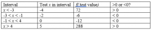
Solve $(x + 3){(x + 1)^2}(x - 4) > 0$

As with all inequalities, we start by solving the equality $(x + 3){(x + 1)^2}(x - 4) = 0$ , which has solutions at x = -3, -1, and 4. We know the function can only change from positive to negative at these values, so these divide the inputs into 4 intervals.

We could choose a test value in each interval and evaluate the function $f(x) = (x + 3){(x + 1)^2}(x - 4)$ at each test value to determine if the function is positive or negative in that interval

On a number line this would look like:

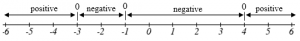
From our test values, we can determine this function is positive when x < -3 or x > 4, or in interval notation, $( - \infty , - 3) \cup (4,\infty )$

We could have also determined on which intervals the function was positive by sketching a graph of the function. We illustrate that technique in the next example.

Example 9.2H: Finding Domain of a Function

Find the domain of the function $v(t) = \sqrt {6 - 5t - {t^2}}$ .

A square root is only defined when the quantity we are taking the square root of, the quantity inside the square root, is zero or greater. Thus, the domain of this function will be when $6 - 5t - {t^2} \ge 0$ .

Again we start by solving the equality $6 - 5t - {t^2} = 0$ . While we could use the quadratic formula, this equation factors nicely to $(6 + t)(1 - t) = 0$ , giving horizontal intercepts t = 1 and t = -6. Sketching a graph of this quadratic will allow us to determine when it is positive.

From the graph we can see this function is positive for inputs between the intercepts. So $6 - 5t - {t^2} \ge 0$ for $- 6 \le t \le 1$ , and this will be the domain of the v(t) function.

Give it Some Thought

2. Given the function $g(x) = {x^3} - {x^2} - 6x$ use the methods that we have learned so far to find the vertical & horizontal intercepts, determine where the function is negative and positive, describe the long run behavior and sketch the graph without technology.

Estimating Extrema

With quadratics, we were able to algebraically find the maximum or minimum value of the function by finding the vertex. For general polynomials, finding these turning points is not possible without more advanced techniques from calculus. Even then, finding where extrema occur can still be algebraically challenging. For now, we will estimate the locations of turning points using technology to generate a graph.

Example 9.2I: Estimating Extrema

An open-top box is to be constructed by cutting out squares from each corner of a 14cm by 20cm sheet of plastic then folding up the sides. Find the size of squares that should be cut out to maximize the volume enclosed by the box.

We will start this problem by drawing a picture, labeling the width of the cut-out squares with a variable, w.

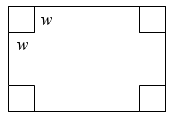
Notice that after a square is cut out from each end, it leaves a (14-2w) cm by (20-2w) cm rectangle for the base of the box, and the box will be w cm tall. This gives the volume:

$V(w) = (14 - 2w)(20 - 2w)w = 280w - 68{w^2} + 4{w^3}$

Using technology to sketch a graph allows us to estimate the maximum value for the volume, restricted to reasonable values for w: values from 0 to 7.

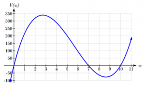
From this graph, we can estimate the maximum value is around 340, and occurs when the squares are about 2.75cm square. To improve this estimate, we could use advanced features of our technology, if available, or simply change our window to zoom in on our graph.

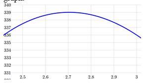
From this zoomed-in view, we can refine our estimate for the max volume to about 339, when the squares are 2.7cm square.

Give It Some Thought

3. Use technology to find the maximum and minimum values on the interval [-1, 4] of the function $f(x) = - 0.2{(x - 2)^3}{(x + 1)^2}(x - 4)$ .

Give It Some Thought Answers

1. Vertical intercept (0, 0), Horizontal intercepts (0, 0), (-2, 0), (2, 0)

2. Vertical intercept (0, 0), Horizontal intercepts (-2, 0), (0, 0), (3, 0)

The function is negative on ( $-{x^p}$ %, -2) and (0, 3)

The function is positive on (-2, 0) and (3, ${x^p}$ %)

The leading term is so as

3. The minimum occurs at approximately the point (0, -6.5), and the maximum occurs at approximately the point (3.5, 7).

Section 7.6 Exercises

Insert review exercises here

9.3 Rational Functions

We will begin this section by looking at another economic concept. In addition to total cost and marginal cost, another metric of costs is average cost.

Average Cost

The average cost of producing q items with a total cost of C(q) is $AC(q) = \frac{{C(q)}}{q}$

Example 9.3A: Finding Average Cost

Suppose that manufacturing an item has fixed costs of $4000 and per-item (marginal) costs of $20 per item. Find the average cost per item when 250 items are produced.

The total cost function is $C(q) = 4000 + 20q$ .

Then average cost is $AC(q) = \frac{{4000 + 20q}}{q}$ .

When 250 items are produced, the average cost per item will be

$AC(250) = \frac{{4000 + 20(250)}}{{250}} = $ 36$

The average cost per item is $36.

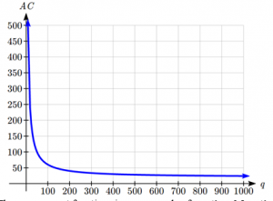
Notice that the average cost per item distributes the fixed costs across all the items. If we were to graph the average cost, notice that average costs decrease as production increases, eventually levelling off towards the per-item cost of $20.

The average cost functions is one example of a rational function.

Rational Functions

A rational function is a function that can be written as the ratio of two polynomials, P(x) and Q(x).

$f(x) = \frac{{P(x)}}{{Q(x)}} = \frac{{{a_0} + {a_1}x + {a_2}{x^2} + \cdots + {a_p}{x^p}}}{{{b_0} + {b_1}x + {b_2}{x^2} + \cdots + {b_q}{x^q}}}$

To get a feel for these functions, we will look at a graph.

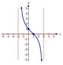
Example 9.3B: Graphing Rational Function

Graph $f(x) = \frac{{2x + 4}}{{x - 3}}$

Notice that the graph is undefined at x = 3, since that would cause us to divide by 0. We can create a table of values to get a sense for the function.

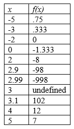
Notice that as x gets close to 3 from the left, the function values are getting larger and larger in the negative direction. When x is close to 3 from the right, the function values are getting large and positive. We call x = 3 a vertical asymptote of the function.

When x = -2, the function value is 0, giving a horizontal intercept. Notice that when x = -2 the numerator of the rational function is zero.

To get a better sense of the long run behavior, we can evaluate the function at additional, larger inputs:

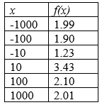
Notice that as x gets large on both ends, the function approaches 2 but never actually reaches 2, it just “levels off” as the inputs become large. This behavior creates a horizontal asymptote. In this case the graph is approaching the horizontal line f(X)=2 as the input becomes very large in the negative and positive directions.

Sketching a graph of this function:

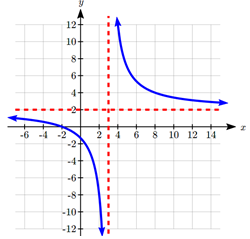
The graphs of rational functions are sometimes sketched with the horizontal and vertical asymptotes drawn as dashed lines. It’s important to realize these are not part of the graph of the function itself.

Vertical and Horizontal Asymptotes

A vertical asymptote of a graph is a vertical line x = a where the graph tends towards positive or negative infinity as the inputs approach a.

A horizontal asymptote of a graph is a horizontal line where the graph approaches the line as the inputs get large.

In the first example looking at average cost, the function had a vertical asymptote at q=0, and a horizontal asymptote at AC=20.

Finding Asymptotes and Intercepts

Given a rational function, as part of investigating the short run behavior we are interested in finding any vertical and horizontal asymptotes, as well as finding any vertical or horizontal intercepts, as we have done in the past.

To find vertical asymptotes, we notice that the vertical asymptotes in our examples occur when the denominator of the function is undefined. With one exception, a vertical asymptote will occur whenever the denominator is undefined.

Example 9.3C: Finding Verical Asymptotes of a Function

Find the vertical asymptotes of the function $k(x) = \frac{{5 + 2{x^2}}}{{2 - x - {x^2}}}$

To find the vertical asymptotes, we determine where this function will be undefined by setting the denominator equal to zero:

$\begin{array}{l} 2 - x - {x^2} = 0\\ (2 + x)(1 - x) = 0\\ x = - 2,\;1 </div> \end{array}$

This indicates two vertical asymptotes, which a look at a graph confirms.

The exception to this rule can occur when both the numerator and denominator of a rational function are zero at the same input.

Example 9.3D: Finding Vertical Asymptotes of a Complex Function

Find the vertical asymptotes of the function $k(x) = \frac{{x - 2}}{{{x^2} - 4}}$ .

To find the vertical asymptotes, we determine where this function will be undefined by setting the denominator equal to zero:

$\begin{array}{l} {x^2} - 4 = 0\\ {x^2} = 4\\ x = - 2,\;2 </div> \end{array}$

However, the numerator of this function is also equal to zero when x = 2. Because of this, the function will still be undefined at 2, since $\frac{0}{0}$ is undefined, but the graph will not have a vertical asymptote at x = 2.

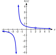
The graph of this function will have the vertical asymptote at x = -2, but at x = 2 the graph will have a hole: a single point where the graph is not defined, indicated by an open circle.

Vertical Asymptotes and Holes of Rational Functions

The vertical asymptotes of a rational function will occur where the denominator of the function is equal to zero and the numerator is not zero.

A hole might occur in the graph of a rational function if an input causes both numerator and denominator to be zero. In this case, factor the numerator and denominator and simplify; if the simplified expression still has a zero in the denominator at the original input the original function has a vertical asymptote at the input, otherwise it has a hole.

To find horizontal asymptotes, we are interested in the behavior of the function as the input grows large, so we consider long run behavior of the numerator and denominator separately. Recall that a polynomial’s long run behavior will mirror that of the leading term. Likewise, a rational function’s long run behavior will mirror that of the ratio of the leading terms of the numerator and denominator functions.

There are three distinct outcomes when this analysis is done:

Case 1: The degree of the denominator > degree of the numerator

Example: $f(x) = \frac{{3x + 2}}{{{x^2} + 4x - 5}}$

In this case, the long run behavior is $f(x) \approx \frac{{3x}}{{{x^2}}} = \frac{3}{x}$ . This tells us that as the inputs grow large, this function will behave similarly to the function $g(x) = \frac{3}{x}$ . As the inputs grow large, the outputs will approach zero, resulting in a horizontal asymptote at y=0.

Case 2: The degree of the denominator < degree of the numerator

Example: $f(x) = \frac{{3{x^2} + 2}}{{x - 5}}$

In this case, the long run behavior is $f(x) \approx \frac{{3{x^2}}}{x} = 3x$ . This tells us that as the inputs grow large, this function will behave similarly to the function $g(x) = 3x$ . As the inputs grow large, the outputs will grow and not level off, so this graph has no horizontal asymptote.

Ultimately, if the numerator is larger than the denominator, the long run behavior of the graph will mimic the behavior of the reduced long run behavior fraction. As another example if we had the function $f(x) = \frac{{3{x^5} - {x^2}}}{{x + 3}}$ with long run behavior $f(x) \approx \frac{{3{x^5}}}{x} = 3{x^4}$ , the long run behavior of the graph would look similar to that of an even polynomial.

Case 3: The degree of the denominator = degree of the numerator

Example: $f(x) = \frac{{3{x^2} + 2}}{{{x^2} + 4x - 5}}$

In this case, the long run behavior is $f(x) \approx \frac{{3{x^2}}}{{{x^2}}} = 3$ . This tells us that as the inputs grow large, this function will behave like the function $g(x) = 3$ , which is a horizontal line. This function has a horizontal asymptote at y=3.

Horizontal Asymptote of Rational Functions

The horizontal asymptote of a rational function can be determined by looking at the degrees of the numerator and denominator.

Degree of denominator > degree of numerator: Horizontal asymptote at y=0

Degree of denominator < degree of numerator: No horizontal asymptote

Degree of denominator = degree of numerator: Horizontal asymptote at ratio of leading coefficients.

Example 9.3E: Finding Horizontal and Vertical Asymptotes of the function

Find the horizontal and vertical asymptotes of the function.

$f(x) = \frac{{(x - 2)(x + 3)}}{{(x - 1)(x + 2)(x - 5)}}$

First, note this function has no inputs that make both the numerator and denominator zero, so there are no potential holes. The function will have vertical asymptotes when the denominator is zero, causing the function to be undefined. The denominator will be zero at x = 1, -2, and 5, indicating vertical asymptotes at these values.

The numerator has degree 2, while the denominator has degree 3. Since the degree of the denominator is greater than the degree of the numerator, the denominator will grow faster than the numerator, causing the outputs to tend towards zero as the inputs get large, and so as $x \to \pm \infty$ , $f(x) \to 0$ . This function will have a horizontal asymptote at y=0.

Give It Some Thought

1. Find the vertical and horizontal asymptotes of the function.

$f(x) = \frac{{(2x - 1)(2x + 1)}}{{(x - 2)(x + 3)}}$

Example 9.3F: Determining Market Share

Nadi Products, an Ebay retailer that resells items purchased from Fiji, has started selling a new-to-market product. Nadi is currently selling 2,000 units a month, which has been growing by 100 units a month. The total market for the product is currently 10,000 units, but is growing by 1000 units a month.

a) Determine Nadi’s current market share.

b) Find the horizontal asymptote and interpret it in context of the scenario.

Notice that the sales per month are increasing linearly. Let t be the number of months, then Nadi’s sales per month are $N = 2000 + 100t$ , and the total market is $M = 10000 + 1000t$ .

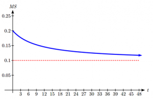
Nadi’s market share, MS, the fraction of the total market that Nadi holds:

$MS(t) = \frac{{2000 + 100t}}{{10000 + 1000t}}$

a) Nadi’s current market share is:

$MS(0) = \frac{{2000 + 100(0)}}{{10000 + 1000(0)}} = \frac{{2000}}{{10000}} = 0.20 = 20\%$

b) Both the numerator and denominator are linear (degree 1), so since the degrees are equal, there will be a horizontal asymptote at the ratio of the leading coefficients. In the numerator, the leading term is 100t, with coefficient 100. In the denominator, the leading term is 1000t, with coefficient 1000. The horizontal asymptote will be at the ratio of these values, at $y = \frac{{100}}{{1000}} = 0.10$ .

This tells us that as the input gets large, the output values will approach 0.10. In context, this means that as more time goes by, Nadi’s market share will approach 10%.

Intercepts

As with all functions, a rational function will have a vertical intercept when the input is zero, if the function is defined at zero. It is possible for a rational function to not have a vertical intercept if the function is undefined at zero.

Likewise, a rational function will have horizontal intercepts at the inputs that cause the output to be zero (unless that input corresponds to a hole). It is possible there are no horizontal intercepts. Since a fraction is only equal to zero when the numerator is zero, horizontal intercepts will occur when the numerator of the rational function is equal to zero.

Example 9.3G: Finding Inercepts by Evaluating the Function at Zero

Find the intercepts of $f(x) = \frac{{(x - 2)(x + 3)}}{{(x - 1)(x + 2)(x - 5)}}$

We can find the vertical intercept by evaluating the function at zero

$f(0) = \frac{{(0 - 2)(0 + 3)}}{{(0 - 1)(0 + 2)(0 - 5)}} = \frac{{ - 6}}{{10}} = - \frac{3}{5}$

The horizontal intercepts will occur when the function is equal to zero:

$0 = \frac{{(x - 2)(x + 3)}}{{(x - 1)(x + 2)(x - 5)}}$ This is zero when the numerator is zero

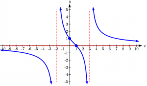
$\begin{array}{l} 0 = (x - 2)(x + 3)\\ x = 2,\; - 3 </div> \end{array}$ %

Example 9.3H: Sketching Graph by Evaluating the Function at Zero

Sketch a graph of $f(x) = \frac{{6(x - 1)}}{{(x + 2)(x - 3)}}$ .

We can start our sketch by finding intercepts and asymptotes. Evaluating the function at zero gives the vertical intercept:

$f(0) = \frac{{6(0 - 1)}}{{(0 + 2)(0 - 3)}} = \frac{{ - 6}}{{ - 6}} = 1$

Looking at when the numerator of the function is zero, we can determine the graph will have a horizontal intercept at x = 1.

Looking at when the denominator of the function is zero, we can determine the graph will have vertical asymptotes at x = -2 and x = 3.

Finally, the degree of denominator is larger than the degree of the numerator, telling us this graph has a horizontal asymptote at y = 0.

To sketch the graph, we might start by plotting the intercepts and drawing the asymptotes as dashed lines.

We can now try to sketch a smooth curve passing through both intercepts. As the graph approaches x=3, the graph must approach negative infinity. As we sketch from x=0 towards x=-2, we’d expect the graph to approach positive infinity.

To finish the curve, we need to fill in the portions to the right of x=3 and to the left of x=-2. If we evaluate the function to the right of x=3 we’d see the output is positive, indicating the graph will decrease from positive infinity then level off towards the horizontal asymptote of y=0. To the left of x=-2 the graph will also level off at the horizontal asymptote, and will approach negative infinity to the left of the asymptote.

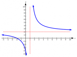
Give It Some Thought

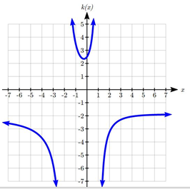
2. Given the function $f(x) = \frac{{2(x + 2)}}{{x - 1}}$ , find the intercepts and asymptotes and sketch the function.

Give It Some Thought Answers

1. Vertical asymptotes at x = 2 and x = -3; horizontal asymptote at y = 4

2. Horizontal asymptote at y = 2.

Vertical asymptote is at x = 1.

Vertical intercept at (0, 4).

Horizontal intercept (2, 0).

Key Takeaways

Section 9.1: Quadratic Functions

Forms f Quadratic Functions
Finding the Vertex of a Quadratic
Maximizing Revenue or Profit
Quadratic Formula

Section 9.2: Domain and Range

Characteristics of Power Functions
Polynomials
Graphical Behavior at Intercepts
Solving Polynomials Inequalities
Estimating Extrema

Section 9.3: Rates of Change and Behaviour of Graphs

Rational Functions
Vertical and Horizontal Asymptotes
Vertical Asymptotes and Holes of Rational Functions
Horizontal Asymptote of Rational Functions
Intercepts

License

Icon for the Creative Commons Attribution-NonCommercial-ShareAlike 4.0 International License

BUSI1915 - Fundamentals of Business Mathematics Copyright © by OER Lab is licensed under a Creative Commons Attribution-NonCommercial-ShareAlike 4.0 International License, except where otherwise noted.

9.1 Quadratic Functions

Short run Behavior: Vertex

Forms of Quadratic Functions

Finding the Vertex of a Quadratic

Maximizing Revenue or Profit

Short run Behavior: Intercepts

Quadratic Formula

Give It Some Thought Answers

9.2 Polynomial Functions

Power Functions

Characteristics of Power Functions

Long Run Behavior

Terminology of Polynomial Functions

Long Run Behavior of Polynomials

Short Run Behavior: Intercepts

Intercepts and Turning Points of Polynomials

Graphical Behavior of Polynomials at Horizontal Intercepts

Solving Polynomial Inequalities

Estimating Extrema

Give It Some Thought Answers

Section 7.6 Exercises

9.3 Rational Functions

Average Cost

Rational Functions

Vertical and Horizontal Asymptotes

Finding Asymptotes and Intercepts

Vertical Asymptotes and Holes of Rational Functions

Horizontal Asymptote of Rational Functions

Intercepts

License

Share This Book