Exponential and Logarithmic Functions

OER Lab

10 Exponential and Logarithmic Functions

Chapter 10 Topics

10.1 Exponential Functions

10.2 Logarithmic Functions

10.3 Exponential and Logarithmic Models

10.1 Exponential Functions

India is the second most populous country in the world, with a population in 2008 of about 1.14 billion people. The population is growing by about 1.34% each year¹. We might ask if we can find a formula to model the population, P, as a function of time, t, in years after 2008, if the population continues to grow at this rate.

In linear growth, we had a constant rate of change – a constant number that the output increased for each increase in input. For example, in the equation $f(x) = 3x + 4$ % , the slope tells us the output increases by three each time the input increases by one. This population scenario is different – we have a percent rate of change rather than a constant number of people as our rate of change. To see the significance of this difference consider these two companies:

Company A has 100 stores, and expands by opening 50 new stores a year

Company B has 100 stores, and expands by increasing the number of stores by 50% of their total each year.

Looking at a few years of growth for these companies:

Year	Stores, company A		Stores, company B
0	100	Starting with 100 each	100
1	100 + 50 = 150	They both grow by 50 stores in the first year.	100 + 50% of 100 100 + 0.50(100) = 150
2	150 + 50 = 200	Store A grows by 50, Store B grows by 75	150 + 50% of 150 150 + 0.50(150) = 225
3	200 + 50 = 250	Store A grows by 50, Store B grows by 112.5	225 + 50% of 225 225 + 0.50(225) = 337.5

Notice that with the percent growth, each year the company is grows by 50% of the current year’s total, so as the company grows larger, the number of stores added in a year grows as well.

To try to simplify the calculations, notice that after 1 year the number of stores for company B was:

$100 + 0.50(100)$

or equivalently by factoring

$100(1 + 0.50) = 150$

We can think of this as “the new number of stores is the original 100% plus another 50%”.

After 2 years, the number of stores was:

$150 + 0.50(150)$

or equivalently by factoring

$150(1 + 0.50)$

now recall the 150 came from 100(1+0.50). Substituting that,

$100(1 + 0.50)(1 + 0.50) = 100{(1 + 0.50)^2} = 225$

After 3 years, the number of stores was:

$225 + 0.50(225)$

or equivalently by factoring

$225(1 + 0.50)$

now recall the 225 came from

$100{(1 + 0.50)^2}$

. Substituting that,

$100{(1 + 0.50)^2}(1 + 0.50) = 100{(1 + 0.50)^3} = 337.5$

From this, we can generalize, noticing that to show a 50% increase, each year we multiply by a factor of (1+0.50), so after n years, our equation would be

$B(n) = 100{(1 + 0.50)^n}$

In this equation, the 100 represented the initial quantity, and the 0.50 was the percent growth rate. Generalizing further, we arrive at the general form of exponential functions.

Exponential Function

An exponential growth or decay function is a function that grows or shrinks at a constant percent growth rate. The equation can be written in the form

$f(x) = a{(1 + r)^x}$ or $f(x) = a{b^x}$ where b = 1+r

Where

a is the initial or starting value of the function

r is the percent growth or decay rate, written as a decimal

b is the growth factor or growth multiplier. Since powers of negative numbers behave strangely, we limit b to positive values.

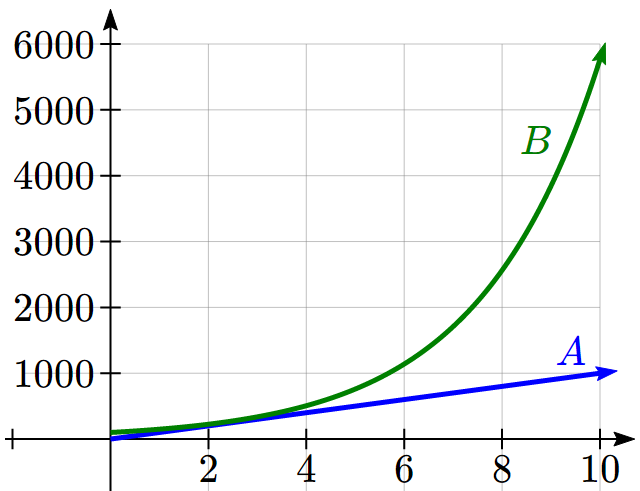
To see more clearly the difference between exponential and linear growth, compare the two tables and graphs below, which illustrate the growth of company A and B described above over a longer time frame if the growth patterns were to continue.

years	Company A	Company B
2	200	225
4	300	506
6	400	1139
8	500	2563
10	600	5767

Example 1

Write an exponential function for India’s population, and use it to predict the population in 2020.

At the beginning of the chapter we were given India’s population of 1.14 billion in the year 2008 and a percent growth rate of 1.34%. Using 2008 as our starting time (t = 0), our initial population will be 1.14 billion. Since the percent growth rate was 1.34%, our value for r is 0.0134.

Using the basic formula for exponential growth

$f(x) = a{(1 + r)^x}$ we can write the formula,

$f(t) = 1.14{(1 + 0.0134)^t}$

To estimate the population in 2020, we evaluate the function at t = 12, since 2020 is 12 years after 2008.

$f(12) = 1.14{(1 + 0.0134)^{12}} \approx 1.337$ billion people in 2020

Try it Now

1. Given the three statements below, identify which represents exponential functions.

A. The cost of living allowance for state employees increases salaries by 3.1% each year.

B. State employees can expect a $300 raise each year they work for the state.

C. Tuition costs have increased by 2.8% each year for the last 3 years.

Example 2

A certificate of deposit (CD) is a type of savings account offered by banks, typically offering a higher interest rate in return for a fixed length of time you will leave your money invested. If a bank offers a 24 month CD with an annual interest rate of 1.2% compounded monthly, how much will a $1000 investment grow to over those 24 months?

First, we must notice that the interest rate is an annual rate, but is compounded monthly, meaning interest is calculated and added to the account monthly.

To find the monthly interest rate, we divide the annual rate of 1.2% by 12 since there are 12 months in a year: 1.2%/12 = 0.1%. Each month we will earn 0.1% interest. From this, we can set up an exponential function, with our initial amount of $1000 and a growth rate of r = 0.001, and our input m measured in months.

$f(m) = 1000{\left( {1 + \frac{{.012}}{{12}}} \right)^m}$

$f(m) = 1000{(1 + 0.001)^m}$

After 24 months, the account will have grown to

$f(24) = 1000{(1 + 0.001)^{24}} = \$ 1024.28$

$B(t) = 900{\left( {1.075} \right)^t}$

Try it Now

2. Looking at these two equations that represent the balance in two different savings accounts, which account is growing faster, and which account will have a higher balance after 3 years?

$A(t) = 1000{\left( {1.05} \right)^t}$

In all the preceding examples, we saw exponential growth. Exponential functions can also be used to model quantities that are decreasing at a constant percent rate. An example of this is radioactive decay, a process in which radioactive isotopes of certain atoms transform to an atom of a different type, causing a percentage decrease of the original material over time.

Example 3

Bismuth-210 is an isotope that radioactively decays by about 13% each day, meaning 13% of the remaining Bismuth-210 transforms into another atom (polonium-210 in this case) each day. If you begin with 100 mg of Bismuth-210, how much remains after one week?

With radioactive decay, instead of the quantity increasing at a percent rate, the quantity is decreasing at a percent rate. Our initial quantity is a = 100 mg, and our growth rate will be negative 13%, since we are decreasing: r = -0.13. This gives the equation:

$Q(d) = 100{(1 - 0.13)^d} = 100{(0.87)^d}$

This can also be explained by recognizing that if 13% decays, then 87 % remains.

After one week, 7 days, the quantity remaining would be

$Q(7) = 100{(0.87)^7} = 37.73$

mg of Bismuth-210 remains.

Try it Now

3. A population of 1000 is decreasing 3% each year. Find the population in 30 years.

Example 4

T(q) represents the total number of Android smart phone contracts, in thousands, held by a certain Verizon store region measured quarterly since January 1, 2010,

Interpret all of the parts of the equation $T(2) = 86{(1.64)^2} = 231.3056$ .

Interpreting this from the basic exponential form, we know that 86 is our initial value. This means that on Jan. 1, 2010 this region had 86,000 Android smart phone contracts. Since b = 1 + r = 1.64, we know that every quarter the number of smart phone contracts grows by 64%. T(2) = 231.3056 means that in the 2^nd quarter (or at the end of the second quarter) there were approximately 231,305 Android smart phone contracts.

Finding Equations of Exponential Functions

In the previous examples, we were able to write equations for exponential functions since we knew the initial quantity and the growth rate. If we do not know the growth rate, but instead know only some input and output pairs of values, we can still construct an exponential function.

Example 5

In 2002, a company had 80 retail stores. By 2008, the company had grown to 180 retail stores. If the company is growing exponentially, find a formula for the function.

By defining our input variable to be t, years after 2002, the information listed can be written as two input-output pairs: (0,80) and (6,180). Notice that by choosing our input variable to be measured as years after the first year value provided, we have effectively “given” ourselves the initial value for the function: a = 80. This gives us an equation of the form

$f(t) = 80{b^t}$ .

Substituting in our second input-output pair allows us to solve for b:

$180 = 80{b^6}$

Divide by 80

${b^6} = \frac{{180}}{{80}} = \frac{9}{4}$

Take the 6^th root of both sides.

$b = \sqrt[6]{{\frac{9}{4}}} = 1.1447$

This gives us our equation for the population:

$f(t) = 80{(1.1447)^t}$

Recall that since b = 1+r, we can interpret this to mean that the population growth rate is r = 0.1447, and so the population is growing by about 14.47% each year.

In this example, you could also have used (9/4)^(1/6) to evaluate the 6^th root if your calculator doesn’t have an n^th root button. We chose to use the $f(x) = a{b^x}$ form of the exponential function rather than the $f(x) = a{(1 + r)^x}$ form, but this choice was entirely arbitrary – either form would be fine to use.

When finding equations, the value for b or r will usually have to be rounded to be written easily. To preserve accuracy, it is important to not over-round these values. Typically, you want to be sure to preserve at least 3 significant digits in the growth rate. For example, if your value for b was 1.00317643, you would want to round this no further than to 1.00318.

Try it now

4. Find the formula for an exponential passing through (0, 10) and (3, 7).

Graphs of Exponentials

To get a sense for the behavior of exponentials, let us begin by looking more closely at the function $f(x) = {2^x}$ .

Listing a table of values for this function:

x	-3	-2	-1	0	1	2	3
f(x)	$\frac{1}{8}$	$\frac{1}{4}$	$\frac{1}{2}$	1	2	4	8

Notice that:

This function is positive for all values of x.
As x increases, the function grows faster and faster (the rate of change increases)
As x decreases, the function values grow smaller, approaching zero.

This is an example of exponential growth.

Looking at the function

$g(x) = {\left( {\frac{1}{2}} \right)^x}$

x	-3	-2	-1	0	1	2	3
g(x)	8	4	2	1	$\frac{1}{2}$	$\frac{1}{4}$	$\frac{1}{8}$

Note this function is also positive for all values of x, but in this case grows as x decreases, and decreases towards zero as x increases. This is an example of exponential decay. You may notice from the table that this function appears to be the horizontal reflection of the $f(x) = {2^x}$ table. This is in fact the case:

$f( - x) = {2^{ - x}} = {({2^{ - 1}})^x} = {\left( {\frac{1}{2}} \right)^x} = g(x)$

Looking at the graphs also confirms this relationship:

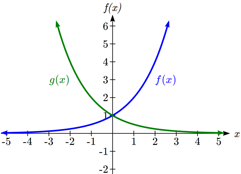
Consider a function for the form $f(x) = a{b^x}$ . Since a, which we called the initial value in the last section, is the function value at an input of zero, a will give us the vertical intercept of the graph. From the graphs above, we can see that an exponential graph will have a horizontal asymptote on one side of the graph, and can either increase or decrease, depending upon the growth factor. This horizontal asymptote will also help us determine the long run behavior and is easy to determine from the graph.

The graph will grow when the growth rate is positive, which will make the growth factor b larger than one. When it’s negative, the growth factor will be less than one.

Graphical Features of Exponential Functions

Graphically, in the function $f(x) = a{b^x}$

a is the vertical intercept of the graph

b determines the rate at which the graph grows. When a is positive,

the function will increase if b > 1

the function will decrease if 0 < b < 1

The graph will have a horizontal asymptote at y = 0

The graph will be concave up if a > 0; concave down if a < 0.

The domain of the function is all real numbers

The range of the function is

$(0,\infty )$

When sketching the graph of an exponential function, it can be helpful to remember that the graph will pass through the points (0, a) and (1, ab).

The value b will determine the function’s long run behavior:

If b > 1, as , and as $x \to \infty$ , $f(x) \to \infty$ and as $x \to - \infty$ , $f(x) \to 0$ .

If 0 < b < 1 , as $x \to \infty$ , $f(x) \to 0$ and as $x \to - \infty$ , $f(x) \to \infty$ .

Example 6

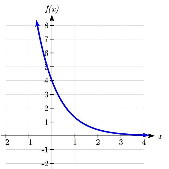
Sketch a graph of $f(x) = 4{\left( {\frac{1}{3}} \right)^x}$

This graph will have a vertical intercept at (0,4), and pass through the point $\left( {1,\frac{4}{3}} \right)$ . Since b < 1, the graph will be decreasing towards zero. Since a > 0, the graph will be concave up.

We can also see from the graph the long run behavior: as , and as , .

To get a better feeling for the effect of a and b on the graph, examine the sets of graphs below. The first set shows various graphs, where a remains the same and we only change the value for b.

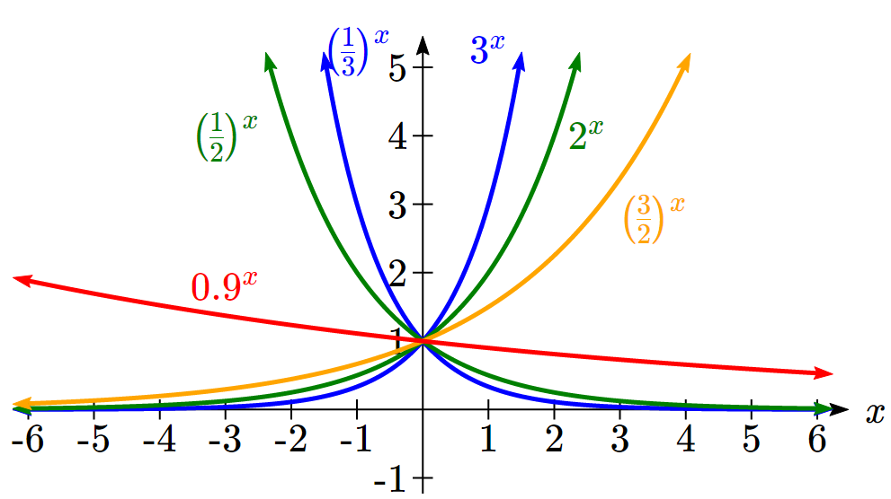
Notice that the closer the value of b is to 1, the less steep the graph will be.

In the next set of graphs, a is altered and our value for b remains the same.

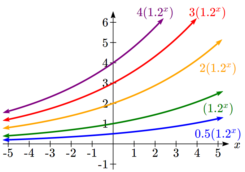
Notice that changing the value for a changes the vertical intercept. Since a is multiplying the b^x term, a acts as a vertical stretch factor, not as a shift. Notice also that the long run behavior for all of these functions is the same because the growth factor did not change and none of these a values introduced a vertical flip.

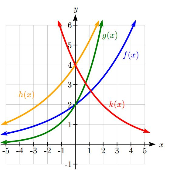
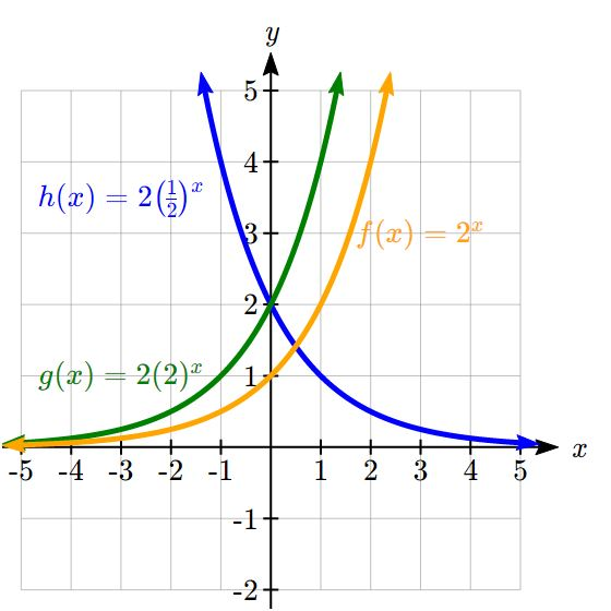
Example 7

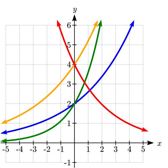
Match each equation with its graph.

$\begin{array}{l} f(x) = 2{(1.3)^x}\\ g(x) = 2{(1.8)^x}\\ h(x) = 4{(1.3)^x}\\ k(x) = 4{(0.7)^x} </div> \end{array}$

The graph of k(x) is the easiest to identify, since it is the only equation with a growth factor less than one, which will produce a decreasing graph. The graph of h(x) can be identified as the only growing exponential function with a vertical intercept at (0,4). The graphs of f(x) and g(x) both have a vertical intercept at (0,2), but since g(x) has a larger growth factor, we can identify it as the graph increasing faster.

Try it now

5. Graph the following functions on the same axis: $f(x) = {(2)^x}$ ; $g(x) = 2{(2)^x}$ ; $h(x) = 2{(1/2)^x}$ .

Compound Interest

In the bank certificate of deposit (CD) example earlier in the section, we encountered compound interest. Typically bank accounts and other savings instruments in which earnings are reinvested, such as mutual funds and retirement accounts, utilize compound interest. The term compounding comes from the behavior that interest is earned not on the original value, but on the accumulated value of the account. We’ll explore compound interest in greater depth in a later chapter, but will introduce basics here.

In the example from earlier, the interest was compounded monthly, so we took the annual interest rate, usually called the nominal rate or annual percentage rate (APR) and divided by 12, the number of compounds in a year, to find the monthly interest. The exponent was then measured in months.

Generalizing this, we can form a general formula for compound interest. If the APR is written in decimal form as r, and there are k compounding periods per year, then the interest per compounding period will be r/k. Likewise, if we are interested in the value after t years, then there will be kt compounding periods in that time.

Compound Interest Formula

Compound Interest can be calculated using the formula

$A(t) = a{\left( {1 + \frac{r}{k}} \right)^{kt}}$

Where

A(t) is the account value

t is measured in years

a is the starting amount of the account, often called the principal

r is the annual percentage rate (APR), also called the nominal rate

k is the number of compounding periods in one year

Example 8

If you invest $3,000 in an investment account paying 3% interest compounded quarterly, how much will the account be worth in 10 years?

Since we are starting with $3000, a = 3000

Our interest rate is 3%, so r = 0.03

Since we are compounding quarterly, we are compounding 4 times per year, so k = 4

We want to know the value of the account in 10 years, so we are looking for A(10), the value when t = 10.

$A(10) = 3000{\left( {1 + \frac{{0.03}}{4}} \right)^{4(10)}} = $ 4045.05$

The account will be worth $4045.05 in 10 years.

Example 9

A 529 plan is a college savings plan in which a relative can invest money to pay for a child’s later college tuition, and the account grows tax free. If Lily wants to set up a 529 account for her new granddaughter, wants the account to grow to $40,000 over 18 years, and she believes the account will earn 6% compounded semi-annually (twice a year), how much will Lily need to invest in the account now?

Since the account is earning 6%, r = 0.06

Since interest is compounded twice a year, k = 2

In this problem, we don’t know how much we are starting with, so we will be solving for a, the initial amount needed. We do know we want the end amount to be $40,000, so we will be looking for the value of a so that A(18) = 40,000.

$\begin{array}{l} 40,000 = A(18) = a{\left( {1 + \frac{{0.06}}{2}} \right)^{2(18)}}\\ 40,000 = a(2.8983)\\ a = \frac{{40,000}}{{2.8983}} \approx $ 13,801 </div> \end{array}$

Lily will need to invest $13,801 to have $40,000 in 18 years.

Try it now

6. Recalculate example 8 from above with monthly compounding.

A Limit to Compounding

Because of compounding throughout the year, with compound interest the actual increase in a year is more than the annual percentage rate. If $1,000 were invested at 10%, the table below shows the value after 1 year at different compounding frequencies:

Frequency	Value after 1 year
Annually	$1100
Semiannually	$1102.50
Quarterly	$1103.81
Monthly	$1104.71
Daily	$11010.16

The amount we earn increases as we increase the compounding frequency. Notice, though, that the increase from annual to semi-annual compounding is larger than the increase from monthly to daily compounding. This might lead us to believe that although increasing the frequency of compounding will increase our result, there is an upper limit to this process.

To see this, let us examine the value of $1 invested at 100% interest for 1 year.

Frequency	Value
Annual	$2
Semiannually	$2.25
Quarterly	$2.441406
Monthly	$2.613035
Daily	$2.714567
Hourly	$2.718127
Once per minute	$2.718279
Once per second	$2.718282

These values do indeed appear to be approaching an upper limit. This value ends up being so important that it gets represented by its own letter, much like how $\pi$ represents a number.

Euler’s Number: e

e is the letter used to represent the value that ${\left( {1 + \frac{1}{k}} \right)^k}$ approaches as k gets big.

$e \approx 2.718282$

Because e is often used as the base of an exponential, most scientific and graphing calculators have a button that can calculate powers of e, usually labeled e^x. Some computer software instead defines a function exp(x), where exp(x) = e^x.

Because e arises when the time between compounds becomes very small, e allows us to define continuous growth and allows us to define a new toolkit function,

$f(x) = {e^x}$

.

Continuous Growth Formula

Continuous Growth can be calculated using the formula

$f(x) = a{e^{rx}}$

where

a is the starting amount

r is the continuous growth rate

This type of equation is commonly used when describing quantities that change more or less continuously, like chemical reactions, growth of large populations, and radioactive decay. It is also used extensively in calculus.

Example 10

Radon-222 decays at a continuous rate of 17.3% per day. How much will 100mg of Radon-222 decay to in 3 days?

Since we are given a continuous decay rate, we use the continuous growth formula. Since the substance is decaying, we know the growth rate will be negative: r = -0.173

$f(3) = 100{e^{ - 0.173(3)}} \approx 59.512$ mg of Radon-222 will remain.

Try it Now

7. Interpret the following: if S(t) represents the growth of a substance in grams, and time is measured in days.

Continuous growth is also often applied to compound interest, allowing us to talk about continuous compounding.

Example 11

If $1000 is invested in an account earning 10% compounded continuously, find the value after 1 year.

Here, the continuous growth rate is 10%, so r = 0.10. We start with $1000, so a = 1000.

To find the value after 1 year,

$f(1) = 1000{e^{0.10(1)}} \approx $ 1105.17$

Notice this is a $1010.17 increase for the year. As a percent increase, this is

$\frac{{105.17}}{{1000}} = 0.10517 = 10.517\%$ increase over the original $1000.

Notice that this value is slightly larger than the amount generated by daily compounding in the table computed earlier.

The continuous growth rate is like the nominal growth rate (or APR) – it reflects the growth rate before compounding takes effect. This is different than the annual growth rate used in the formula $f(x) = a{(1 + r)^x}$ , which is like the annual percentage yield – it reflects the actual amount the output grows in a year.

While the continuous growth rate in the example above was 10%, the actual annual yield was 10.517%. This means we could write two different looking but equivalent formulas for this account’s growth:

$f(t) = 1000{e^{0.10t}}$

using the 10% continuous growth rate

$f(t) = 1000{(1.10517)^t}$

using the 10.517% actual annual yield rate.

Key Takeaways

Percent growth

Exponential functions

Finding formulas

Interpreting equations

Graphs – Intercept and Growth factor

Exponential Growth & Decay

Long run behavior

Compound interest

Continuous Growth

Try it Now Answers

1. A & C are exponential functions, they grow by a % not a constant number.

2. B(t) is growing faster, but after 3 years A(t) still has a higher account balance

3. , or about 401 people.

4.

$f(x) = 10{(0.8879)^x}$

.

5.

6. $4048.06

7. An initial substance weighing 20g is growing at a continuous rate of 12% per day.

10.2 Logarithmic Functions

A population of 50 flies is expected to double every week, leading to a function of the form $f(x) = 50{(2)^x}$ , where x represents the number of weeks that have passed. When will this population reach 500? Trying to solve this problem leads to:

$500 = 50{(2)^x}$

Dividing both sides by 50 to isolate the exponential

$10 = {2^x}$

While we have set up exponential models and used them to make predictions, you may have noticed that solving exponential equations has not yet been mentioned. The reason is simple: none of the algebraic tools discussed so far are sufficient to solve exponential equations. Consider the equation ${2^x} = 10$

above. We know that ${2^3} = 8$ and ${2^4} = 16$ %, so it is clear that x must be some value between 3 and 4 since

$g(x) = {2^x}$

is increasing. We could use technology to create a table of values or graph to better estimate the solution.

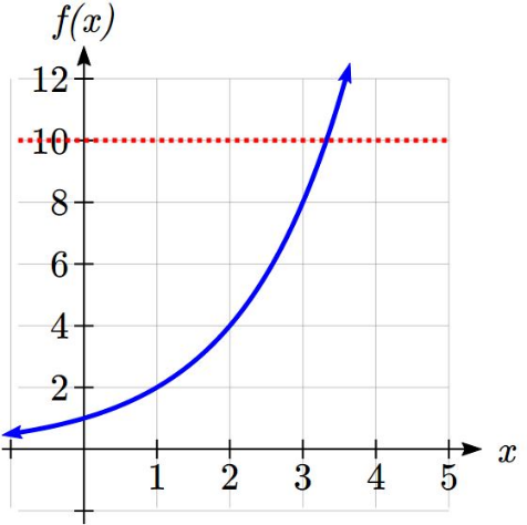
From the graph, we could better estimate the solution to be around 3.3. This result is still fairly unsatisfactory, since it would be nice to have a function that gives the answer. None of the functions we have already discussed would work, so we must introduce a new function, named log, as the function that “undoes” an exponential function, like how a square root “undoes” a square. Since exponential functions have different bases, we will define corresponding logarithms of different bases as well.

Logarithm

The logarithm (base b) function, written ${\log _b}\left( x \right)$ , “undoes” exponential function

${b^x}$

.

The statement ${b^a} = c$ is equivalent to the statement ${\log _b}(c) = a$ .

Since the logarithm and exponential “undo” each other (in technical terms, they are inverses), it follows that:

Properties of Logs: Inverse Properties

${\log _b}\left( {{b^x}} \right) = x$

${b^{{{\log }_b}x}} = x$

Since log is a function, it is most correctly written as ${\log _b}(c)$ , using parentheses to denote function evaluation, just as we would with f(c). However, when the input is a single variable or number, it is common to see the parentheses dropped and the expression written as ${\log _b}c$ .

Example 1

Write these exponential equations as logarithmic equations:

${2^3} = 8$ ${5^2} = 25$ ${10^{ - 4}} = \frac{1}{{10000}}$

${\log _2}(8) = 3$ is equivalent to ${2^3} = 8$

${5^2} = 25$ is equivalent to ${\log _5}(25) = 2$

${10^{ - 4}} = \frac{1}{{10000}}$ is equivalent to $lo{g_{10}}\left( {\frac{1}{{10000}}} \right) = - 4$

Example 2

Write these logarithmic equations as exponential equations:

${\log _6}\left( {\sqrt 6 } \right) = \frac{1}{2}$ ${\log _3}\left( 9 \right) = 2$

${\log _6}\left( {\sqrt 6 } \right) = \frac{1}{2}$ is equivalent to ${6^{1/2}} = \sqrt 6$

${\log _3}\left( 9 \right) = 2$ is equivalent to ${3^2} = 9$

Try it Now

1. Write the exponential equation ${4^2} = 16$ as a logarithmic equation.

By establishing the relationship between exponential and logarithmic functions, we can now solve basic logarithmic and exponential equations by rewriting.

Example 3

Solve ${\log _4}\left( x \right) = 2$ for x.

By rewriting this expression as an exponential, ${4^2} = x$ , so x = 16

Example 4

Solve ${2^x} = 10$ for x.

By rewriting this expression as a logarithm, we get $x = {\log _2}(10)$

While this does define a solution, and an exact solution at that, you may find it somewhat unsatisfying since it is difficult to compare this expression to the decimal estimate we made earlier. Also, giving an exact expression for a solution is not always useful – often we really need a decimal approximation to the solution. Luckily, this is a task calculators and computers are quite adept at. Unluckily for us, most calculators and computers will only evaluate logarithms of two bases. Happily, this ends up not being a problem, as we’ll see briefly.

Common and Natural Logarithms

The common log is the logarithm with base 10, and is typically written $\log (x)$ .

The natural log is the logarithm with base e, and is typically written $\ln (x)$ .

Example 5

Evaluate $\log (1000)$ using the definition of the common log.

Values of the Common Log

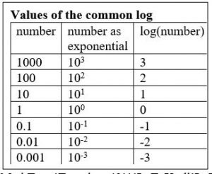
To evaluate $\log(1000)$ , we can say $x = \log(1000)$ , then rewrite into exponential form using the common log base of 10.

${10^x} = 1000$

From this, we might recognize that 1000 is the cube of 10, so x = 3.

We also can use the inverse property of logs to write ${\log _{10}}\left( {{{10}^3}} \right) = 3$

Try it Now

2. Evaluate $\log (1,000,000)$ .

Example 6

Evaluate $\ln \left( {\sqrt e } \right)$ .

We can rewrite $\ln \left( {\sqrt e } \right)$ as $\ln \left( {{e^{1/2}}} \right)$ . Since ln is a log base e, we can use the inverse property for logs: $\ln \left( {{e^{1/2}}} \right) = {\log _e}\left( {{e^{1/2}}} \right) = \frac{1}{2}$ .

Example 7

Evaluate log(500) using your calculator or computer.

Using a computer, we can evaluate $\log (500) \approx 2.69897$ .

Graphs of Logarithms

Recall that the exponential function produces this table of values

x	-3	-2	-1	0	1	2	3
f(x)	$\frac{1}{8}$	$\frac{1}{4}$	$\frac{1}{2}$	1	2	4	8

Since the logarithmic function “undoes” the exponential, produces the table of values

x	$\frac{1}{8}$	$\frac{1}{4}$	$\frac{1}{2}$	1	2	4	8
g(x)	-3	-2	-1	0	1	2	3

In this second table, notice that

As the input increases, the output increases.
As input increases, the output increases more slowly.
Since the exponential function only outputs positive values, the logarithm can only accept positive values as inputs, so the domain of the log function is $(0,\infty )$ .
Since the exponential function can accept all real numbers as inputs, the logarithm can output any real number, so the range is all real numbers or $( - \infty ,\infty )$ .

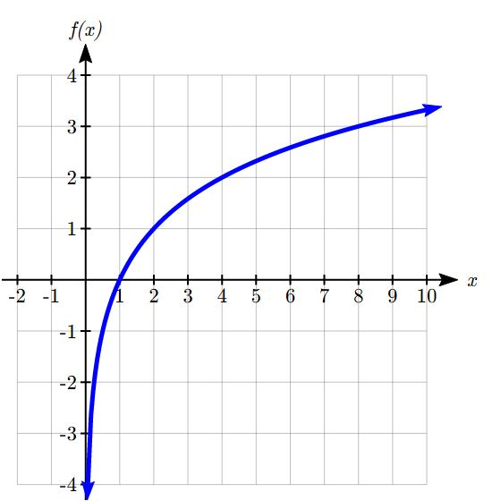
Sketching the graph, notice that as the input approaches zero from the right, the output of the function grows very large in the negative direction, indicating a vertical asymptote at x = 0.

In symbolic notation, we write

as $x \to {0^ + },f(x) \to - \infty$ , and as $x \to \infty ,f(x) \to \infty$

Graphical Features of the Logarithm

Graphically, in the function $g(x) = lo{g_b}(x)$

The graph has a horizontal intercept at (1, 0)

The graph has a vertical asymptote at x = 0

The graph is increasing and concave down

The domain of the function is x > 0, or $(0,\infty )$

The range of the function is all real numbers, or $( - \infty ,\infty )$

When sketching a general logarithm with base b, it can be helpful to remember that the graph will pass through the points (1, 0) and (b, 1).

To get a feeling for how the base affects the shape of the graph, examine the graphs below.

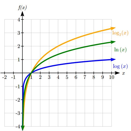
Notice that the larger the base, the slower the graph grows. For example, the common log graph, while it grows without bound, it does so very slowly. For example, to reach an output of 8, the input must be 100,000,000.

Another important observation made was the domain of the logarithm. Like the reciprocal and square root functions, the logarithm has a restricted domain which must be considered when finding the domain of a composition involving a log.

Example 8

Find the domain of the function $f(x) = \log (5 - 2x)$

The logarithm is only defined with the input is positive, so this function will only be defined when $5 - 2x > 0$ .

$\begin{array}{l} - 2x > - 5\\ x < \frac{5}{2} </div> \end{array}$ % Solving this inequality,

The domain of this function is $x < \frac{5}{2}$ , or in interval notation, $\left( { - \infty ,\frac{5}{2}} \right)$ .

Logarithm Properties

To utilize the common or natural logarithm functions to evaluate expressions like ${\log _2}(10)$ , we need to establish some additional properties.

Properties of Logs: Exponent Property

${\log _b}\left( {{A^r}} \right) = r{\log _b}\left( A \right)$

To show why this is true, we offer a proof.

Since the logarithmic and exponential functions are inverses,

${b^{{{\log }_b}A}} = A$ % .

So ${A^r} = {\left( {{b^{{{\log }_b}A}}} \right)^r}$

Utilizing the exponential rule that states ${\left( {{x^p}} \right)^q} = {x^{pq}}$ , ${A^r} = {\left( {{b^{{{\log }_b}A}}} \right)^r} = {b^{r{{\log }_b}A}}$

So then ${\log _b}\left( {{A^r}} \right) = {\log _b}\left( {{b^{r{{\log }_b}A}}} \right)$

Again utilizing the inverse property on the right side yields the result ${\log _b}\left( {{A^r}} \right) = r{\log _b}A$

Example 9

Rewrite ${\log _3}\left( {25} \right)$ using the exponent property for logs.

Since 25 = 5², ${\log _3}\left( {25} \right) = {\log _3}\left( {{5^2}} \right) = 2{\log _3}5$

Example 10

Rewrite $4\ln (x)$ using the exponent property for logs.

Using the property in reverse, $4\ln (x) = \ln \left( {{x^4}} \right)$

Try it Now

3. Rewrite using the exponent property for logs: $\ln \left( {\frac{1}{{{x^2}}}} \right)$ .

The exponent property allows us to find a method for changing the base of a logarithmic expression.

Properties of Logs: Change of Base

${\log _b}\left( A \right) = \frac{{{{\log }_c}(A)}}{{{{\log }_c}(b)}}$

Proof:

Let ${\log _b}\left( A \right) = x$ . Rewriting as an exponential gives ${b^x} = A$ . Taking the log base c of both sides of this equation gives ${\log _c}{b^x} = {\log _c}A$

Now utilizing the exponent property for logs on the left side, $x{\log _c}b = {\log _c}A$

Dividing, we obtain $x = \frac{{{{\log }_c}A}}{{{{\log }_c}b}}$

or replacing our expression for x, ${\log _b}A = \frac{{{{\log }_c}A}}{{{{\log }_c}b}}$

With this change of base formula, we can finally find a good decimal approximation to our question from the beginning of the section.

Example 11

Evaluate ${\log _2}(10)$ using the change of base formula.

According to the change of base formula, we can rewrite the log base 2 as a logarithm of any other base. Since our calculators can evaluate the natural log, we might choose to use the natural logarithm, which is the log base e:

${\log _2}10 = \frac{{{{\log }_e}10}}{{{{\log }_e}2}} = \frac{{\ln 10}}{{\ln 2}}$

Using our calculators to evaluate this, $\frac{{\ln 10}}{{\ln 2}} \approx \frac{{2.30259}}{{0.69315}} \approx 3.3219$

This finally allows us to answer our original question – the population of flies we discussed at the beginning of the section will take 3.32 weeks to grow to 500

.

Example 12

Evaluate ${\log _5}(100)$ using the change of base formula.

We can rewrite this expression using any other base. If our calculators are able to evaluate the common logarithm, we could rewrite using the common log, base 10.

${\log _5}(100) = \frac{{{{\log }_{10}}100}}{{{{\log }_{10}}5}} \approx \frac{2}{{0.69897}} = 2.861$

While we were able to solve the basic exponential equation ${2^x} = 10$ by rewriting in logarithmic form and then using the change of base formula to evaluate the logarithm, the proof of the change of base formula illuminates an alternative approach to solving exponential equations.

Solving exponential equations:

Isolate the exponential expressions when possible

Take the logarithm of both sides

Utilize the exponent property for logarithms to pull the variable out of the exponent

Use algebra to solve for the variable.

Example 13

Solve ${2^x} = 10$ for x.

Using this alternative approach, rather than rewrite this exponential into logarithmic form, we will take the logarithm of both sides of the equation. Since we often wish to evaluate the result to a decimal answer, we will usually utilize either the common log or natural log. For this example, we’ll use the natural log:

$\ln \left( {{2^x}} \right) = \ln (10)$

Utilizing the exponent property for logs, $x\ln \left( 2 \right) = \ln (10)$

Now dividing by ln(2), $x = \frac{{ln(10)}}{{ln\left( 2 \right)}} \approx 2.861$

Notice that this result matches the result we found using the change of base formula.

Example 14

In the first section, we predicted the population (in billions) of India t years after 2008 by using the function $f(t) = 1.14{(1 + 0.0134)^t}$ . If the population continues following this trend, when will the population reach 2 billion?

We need to solve for the t so that f(t) = 2

$2 = 1.14{(1.0134)^t}$

Divide by 1.14 to isolate the exponential expression

$\frac{2}{{1.14}} = {1.0134^t}$

Take the logarithm of both sides of the equation

$\ln \left( {\frac{2}{{1.14}}} \right) = \ln \left( {{{1.0134}^t}} \right)$

Apply the exponent property on the right side

$\ln \left( {\frac{2}{{1.14}}} \right) = t\ln \left( {1.0134} \right)$

Divide both sides by ln(1.0134)

$t = \frac{{\ln \left( {\frac{2}{{1.14}}} \right)}}{{\ln \left( {1.0134} \right)}} \approx 42.23$

years

If this growth rate continues, the model predicts the population of India will reach 2 billion about 42 years after 2008, or approximately in the year 2050.

Try it now

4. Solve $5{(0.93)^x} = 10$ .

Additional Properties of Logarithms

Some situations cannot be addressed using the properties already discussed. For these, we need some additional properties.

Properties of Logs

Sum of Logs Property: ${\log _b}\left( A \right) + {\log _b}\left( C \right) = {\log _b}(AC)$

Difference of Logs Property: ${\log _b}\left( A \right) - {\log _b}\left( C \right) = {\log _b}\left( {\frac{A}{C}} \right)$

It’s just as important to know what properties logarithms do not satisfy as to memorize the valid properties listed above. In particular, the logarithm is not a linear function, which means that it does not distribute: log(A + B) ≠ log(A) + log(B).

With these properties, we can rewrite expressions involving multiple logs as a single log, or break an expression involving a single log into expressions involving multiple logs.

Example 15

Write ${\log _3}\left( 5 \right) + {\log _3}\left( 8 \right) - {\log _3}\left( 2 \right)$ as a single logarithm.

Using the sum of logs property on the first two terms,

${\log _3}\left( 5 \right) + {\log _3}\left( 8 \right) = {\log _3}\left( {5 \cdot 8} \right) = {\log _3}\left( {40} \right)$

This reduces our original expression to ${\log _3}\left( {40} \right) - {\log _3}\left( 2 \right)$

Then using the difference of logs property,

${\log _3}\left( {40} \right) - {\log _3}\left( 2 \right) = {\log _3}\left( {\frac{{40}}{2}} \right) = {\log _3}\left( {20} \right)$

Example 16

Evaluate $2\log \left( 5 \right) + \log \left( 4 \right)$ without a calculator by first rewriting as a single logarithm.

On the first term, we can use the exponent property of logs to write $2\log \left( 5 \right) = \log \left( {{5^2}} \right) = \log \left( {25} \right)$

With the expression reduced to a sum of two logs, $\log \left( {25} \right) + \log \left( 4 \right)$ , we can utilize the sum of logs property $\log \left( {25} \right) + \log \left( 4 \right) = \log (4 \cdot 25) = \log (100)$

Since 100 = 10², we can evaluate this log without a calculator:

$\log (100) = \log \left( {{{10}^2}} \right) = 2$

Example 17

Rewrite $\ln \left( {\frac{{{x^4}y}}{7}} \right)$ as a sum or difference of logs

First, noticing we have a quotient of two expressions, we can utilize the difference property of logs to write $\ln \left( {\frac{{{x^4}y}}{7}} \right) = \ln \left( {{x^4}y} \right) - \ln (7)$

Then seeing the product in the first term, we use the sum property $\ln \left( {{x^4}y} \right) - \ln (7) = \ln \left( {{x^4}} \right) + \ln (y) - \ln (7)$

Finally, we could use the exponent property on the first term $\ln \left( {{x^4}} \right) + \ln (y) - \ln (7) = 4\ln (x) + \ln (y) - \ln (7)$

Try it Now

5. Without a calculator evaluate by first rewriting as a single logarithm ${\log _2}\left( 8 \right) + {\log _2}\left( 4 \right)$ :

Log properties in solving equations

The logarithm properties often arise when solving problems involving logarithms.

Example 18

Solve $\log (50x + 25) - \log (x) = 2$ .

In order to rewrite in exponential form, we need a single logarithmic expression on the left side of the equation. Using the difference property of logs, we can rewrite the left side:

$\log \left( {\frac{{50x + 25}}{x}} \right) = 2$

Rewriting in exponential form reduces this to an algebraic equation:

$\frac{{50x + 25}}{x} = {10^2} = 100$

Solving,

$\begin{array}{l} 50x + 25 = 100x\\ 25 = 50x\\ x = \frac{{25}}{{50}} = \frac{1}{2} </div> \end{array}$

Checking this answer in the original equation, we can verify there are no domain issues, and this answer is correct.

Try it Now

6. Solve $\log ({x^2} - 4) = 1 + \log (x + 2)$ .

Key Takeaways

The Logarithmic function as the inverse of the exponential function

Writing logarithmic & exponential expressions

Properties of logs

Inverse properties

Exponent property

Change of base

Sum and difference of logs properties

Common log

Natural log

Graph of the logarithmic function (domain and range)

Solving exponential equations

Solving equations using log rules

Try it Now Answers

1.

2. 6

3.

4.

5. 5

6. 12

10.3 Exponential and Logarithmic Models

While we have explored some basic applications of exponential and logarithmic functions, in this section we explore some important applications in more depth.

More complex exponential equations can often be solved in more than one way. In the following example, we will solve the same problem in two ways – one using logarithm properties, and the other using exponential properties.

Example 1a

In 2008, the population of Kenya was approximately 38.8 million, and was growing by 2.64% each year, while the population of Sudan was approximately 41.3 million and growing by 2.24% each year². If these trends continue, when will the population of Kenya match that of Sudan?

We start by writing an equation for each population in terms of t, the number of years after 2008.

$\begin{array}{l} Kenya(t) = 38.8{(1 + 0.0264)^t}\\ Sudan(t) = 41.3{(1 + 0.0224)^t} </div> \end{array}$

To find when the populations will be equal, we can set the equations equal

$38.8{(1.0264)^t} = 41.3{(1.0224)^t}$

For our first approach, we take the log of both sides of the equation

$log\left( {38.8{{(1.0264)}^t}} \right) = log\left( {41.3{{(1.0224)}^t}} \right)$

Utilizing the sum property of logs, we can rewrite each side,

$log(38.8) + log\left( {{{1.0264}^t}} \right) = log(41.3) + log\left( {{{1.0224}^t}} \right)$

Then utilizing the exponent property, we can pull the variables out of the exponent $log(38.8) + tlog\left( {1.0264} \right) = log(41.3) + tlog\left( {1.0224} \right)$

Moving all the terms involving t to one side of the equation and the rest of the terms to the other side, $tlog\left( {1.0264} \right) - tlog\left( {1.0224} \right) = log(41.3) - log(38.8)$

Factoring out the t on the left,

$t\left( {log\left( {1.0264} \right) - log\left( {1.0224} \right)} \right) = log(41.3) - log(38.8)$

Dividing to solve for t

$t = \frac{{log(41.3) - log(38.8)}}{{log\left( {1.0264} \right) - log\left( {1.0224} \right)}} \approx 15.991$

years until the populations will be equal.

Example 1b

Solve the problem above by rewriting before taking the log.

Starting at the equation $38.8{(1.0264)^t} = 41.3{(1.0224)^t}$

Divide to move the exponential terms to one side of the equation and the constants to the other side $\frac{{{{1.0264}^t}}}{{{{1.0224}^t}}} = \frac{{41.3}}{{38.8}}$

Using exponent rules to group on the left, ${\left( {\frac{{1.0264}}{{1.0224}}} \right)^t} = \frac{{41.3}}{{38.8}}$

Taking the log of both sides $log\left( {{{\left( {\frac{{1.0264}}{{1.0224}}} \right)}^t}} \right) = log\left( {\frac{{41.3}}{{38.8}}} \right)$

Utilizing the exponent property on the left, $tlog\left( {\frac{{1.0264}}{{1.0224}}} \right) = log\left( {\frac{{41.3}}{{38.8}}} \right)$

Dividing gives $t = \frac{{log\left( {\frac{{41.3}}{{38.8}}} \right)}}{{log\left( {\frac{{1.0264}}{{1.0224}}} \right)}} \approx 15.991$

years

While the answer does not immediately appear identical to that produced using the previous method, note that by using the difference property of logs, the answer could be rewritten:

$t = \frac{{log\left( {\fr<span style="font-size: 1em">ac{{41.</span><span style="font-size: 1em">3}}{{38.8}}} \right)}}{{log\left( {\frac{{1.0264}}{{1.0224}}} \right)}} = \frac{{log(41.3) - log(38.8)}}{{log(1.0264) - log(1.0224)}}$

While both methods work equally well, it often requires fewer steps to utilize algebra before taking logs, rather than relying solely on log properties.

Try it Now

1. Tank A contains 10 liters of water, and 35% of the water evaporates each week. Tank B contains 30 liters of water, and 50% of the water evaporates each week. In how many weeks will the tanks contain the same amount of water?

Radioactive Decay

In an earlier section, we discussed radioactive decay – the idea that radioactive isotopes change over time. One of the common terms associated with radioactive decay is half-life.

Half Life

The half-life of a radioactive isotope is the time it takes for half the substance to decay.

Given the basic exponential growth/decay equation $h(t) = a{b^t}$ , the half-life can be found by solving for when half the original amount remains; by solving $\frac{1}{2}a = a{(b)^t}$ , or more simply $\frac{1}{2} = {b^t}$ . Notice how the initial amount is irrelevant when solving for half-life.

Example 2

Bismuth-210 is an isotope that decays by about 13% each day. What is the half-life of Bismuth-210?

We were not given a starting quantity, so we could either make up a value or use an unknown constant to represent the starting amount. To show that starting quantity does not affect the result, let us denote the initial quantity by the constant a. Then the decay of Bismuth-210 can be described by the equation $Q(d) = a{(0.87)^d}$ .

To find the half-life, we want to determine when the remaining quantity is half the original:

$\frac{1}{2}a$

Solving, $\frac{1}{2}a = a{(0.87)^d}$

Dividing by a, $\frac{1}{2} = {0.87^d}$

Take the log of both sides $\log \left( {\frac{1}{2}} \right) = \log \left( {{{0.87}^d}} \right)$

Use the exponent property of logs

$\log \left( {\frac{1}{2}} \right) = d\log \left( {0.87} \right)$

Divide to solve for d

$d = \frac{{log\left( {\frac{1}{2}} \right)}}{{log\left( {0.87} \right)}} \approx 4.977$

days

This tells us that the half-life of Bismuth-210 is approximately 5 days.

Example 3

Cesium-137 has a half-life of about 30 years. If you begin with 200mg of cesium-137, how much will remain after 30 years? 60 years? 90 years?

Since the half-life is 30 years, after 30 years, half the original amount, 100mg, will remain.

After 60 years, another 30 years have passed, so during that second 30 years, another half of the substance will decay, leaving 50mg.

After 90 years, another 30 years have passed, so another half of the substance will decay, leaving 25mg.

Example 4

Carbon-14 is a radioactive isotope that is present in organic materials, and is commonly used for dating historical artifacts. Carbon-14 has a half-life of 5730 years. If a bone fragment is found that contains 20% of its original carbon-14, how old is the bone?

To find how old the bone is, we first will need to find an equation for the decay of the carbon-14. We could either use a continuous or annual decay formula, but opt to use the continuous decay formula since it is more common in scientific texts. The half life tells us that after 5730 years, half the original substance remains. Solving for the rate, $\frac{1}{2}a = a{e^{r5730}}$

Dividing by a $\frac{1}{2} = {e^{r5730}}$

Taking the natural log of both sides $\ln \left( {\frac{1}{2}} \right) = \ln \left( {{e^{r5730}}} \right)$

Use the inverse property of logs on the right side $\ln \left( {\frac{1}{2}} \right) = 5730r$

Divide by 5730

$r = \frac{{\ln \left( {\frac{1}{2}} \right)}}{{5730}} \approx - 0.000121$

Now we know the decay will follow the equation $Q(t) = a{e^{ - 0.000121t}}$ . To find how old the bone fragment is that contains 20% of the original amount, we solve for t so that Q(t) = 0.20a. $0.20a = a{e^{ - 0.000121t}}$

$0.20 = {e^{ - 0.000121t}}$

$\ln (0.20) = \ln \left( {{e^{ - 0.000121t}}} \right)$

$\ln (0.20) = - 0.000121t$

$t = \frac{{\ln (0.20)}}{{ - 0.000121}} \approx 13301$

years

The bone fragment is about 13,300 years old.

Try it Now

2. In Example 3, we learned that Cesium-137 has a half-life of about 30 years. If you begin with 200mg of cesium-137, how long will it take until only 1 milligram remains?

For decaying quantities, we asked how long it takes for half the substance to decay. For growing quantities we might ask how long it takes for the quantity to double.

Doubling Time

The doubling time of a growing quantity is the time it takes for the quantity to double.

Given the basic exponential growth equation $h(t) = a{b^t}$ , doubling time can be found by solving for when the original quantity has doubled; by solving $2a = a{(b)^x}$ , or more simply $2 = {b^x}$ . Again notice how the initial amount is irrelevant when solving for doubling time.

Example 5

If you invest money at 8% compounded quarterly, how long will it take your money to double?

Using the compound interest equation, we can write $A(t) = P{\left( {1 + \frac{{0.08}}{4}} \right)^{4t}} = P{(1.02)^{4t}}$ .

To find the doubling time, we look for the time until we have twice the original amount, so when A(t) = 2P. Notice we don’t need to know how much was invested.

$2P = P{(1.02)^{4t}}$

$2 = {(1.02)^{4t}}$

$\log \left( 2 \right) = \log \left( {{{1.02}^{4t}}} \right)$

$\log \left( 2 \right) = 4t\log \left( {1.02} \right)$

$t = \frac{{\log \left( 2 \right)}}{{4\log \left( {1.02} \right)}} \approx 8.751$

years.

It will take about 8.75 years for the investment double in value.

Example 6

Use of a new social networking website has been growing exponentially, with the number of new members doubling every 5 months. If the site currently has 120,000 users and this trend continues, how many users will the site have in 1 year?

We can use the doubling time to find a function that models the number of site users, and then use that equation to answer the question. While we could use an arbitrary a as we have before for the initial amount, in this case, we know the initial amount was 120,000.

If we use a continuous growth equation, it would look like $N(t) = 120{e^{rt}}$ , measured in thousands of users after t months. Based on the doubling time, there would be 240 thousand users after 5 months. This allows us to solve for the continuous growth rate:

$240 = 120{e^{r5}}$

$2 = {e^{r5}}$

$\ln 2 = 5r$

$r = \frac{{\ln 2}}{5} \approx 0.1386$

Now that we have an equation, $N(t) = 120{e^{0.1386t}}$ , we can predict the number of users after 12 months: $N(12) = 120{e^{0.1386(12)}} = 633.140$

thousand users.

So after 1 year, we would expect the site to have around 633,140 users.

Try it Now

3. If tuition at a college is increasing by 6.6% each year, how many years will it take for tuition to double?

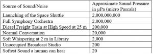
Logarithmic Scales

For quantities that vary greatly in magnitude, a standard linear scale of measurement is not always effective, and utilizing logarithms can make the values more manageable. For example, if the average distances from the sun to the major bodies in our solar system are listed, you see they vary greatly.

Planet	Distance (millions of km)
Mercury	58
Venus	108
Earth	150
Mars	228
Jupiter	779
Saturn	1430
Uranus	2880
Neptune	4500

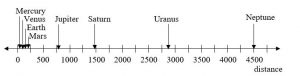
Placed on a linear scale – one with equally spaced values – these values get bunched up.

Distance of planets on the linear scale

However, computing the logarithm of each value and plotting these new values on a number line results in a more manageable graph, and makes the relative distances more apparent.

Planet	Distance (millions of km)	log(distance)
Mercury	58	1.76
Venus	108	2.03
Earth	150	2.18
Mars	228	2.36
Jupiter	779	2.89
Saturn	1430	3.16
Uranus	2880	3.46
Neptune	4500	3.65

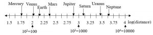
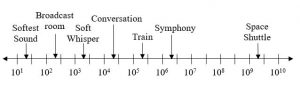
Distance of planets on the Logarithmic scale

Sometimes, as shown above, the scale on a logarithmic number line will show the log values, but more commonly the original values are listed as powers of 10, as shown below.

Example 7

Estimate the value of point P on the log scale above

The point P appears to be half way between -2 and -1 in log value, so if V is the value of this point, $\log (V) \approx - 1.5$

Rewriting in exponential form,

$V \approx {10^{ - 1.5}} = 0.0316$

Example 8

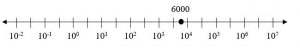
Place the number 6000 on a logarithmic scale.

Since $\log (6000) \approx 3.8$ , this point would belong on the log scale about here:

log(6000) on the log scale

Try it Now

4. Plot the data in the table below on a logarithmic scale³.

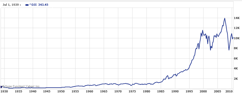
It is also common to see two dimensional graphs with one or both axes using a logarithmic scale. One common use of a logarithmic scale on the vertical axis is to graph quantities that are changing exponentially, since it helps reveal relative differences. This is commonly used in stock charts, since values historically have grown exponentially over time. Both stock charts below show the Dow Jones Industrial Average, from 1928 to 2010.

Linear scale:

Logarithmic scale:

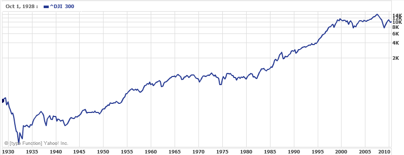
Both charts have a linear horizontal scale, but the first graph has a linear vertical scale, while the second has a logarithmic vertical scale. The first scale is the one we are more familiar with, and shows what appears to be a strong exponential trend, at least up until the year 2000.

Example 9

There were stock market drops in 1929 and 2008. Which was larger?

In the first graph, the stock market drop around 2008 looks very large, and in terms of dollar values, it was indeed a large drop. However the second graph shows relative changes, and the drop in 2009 seems less major on this graph, and in fact the drop starting in 1929 was, percentage-wise, much more significant.

Specifically, in 2008, the Dow value dropped from about 14,000 to 8,000, a drop of 6,000. This is obviously a large value drop, and amounts to about a 43% drop. In 1929, the Dow value dropped from a high of around 380 to a low of 42 by July of 1932. While value-wise this drop of 338 is much smaller than the 2008 drop, it corresponds to a 89% drop, a much larger relative drop than in 2008. The logarithmic scale shows these relative changes

.

Key Takeaway

Radioactive decay

Half life

Doubling time

Logarithmic Scales

Try it Now Answers

1. 4.1874 weeks

2. 229.3157 , or approximately 229 years

3. It will take 10.845 years, or approximately 11 years, for tuition to double.

4.

1 World Bank, World Development Indicators, as reported on http://www.google.com/publicdata, retrieved August 20, 2010

2 World Bank, World Development Indicators, as reported on http://www.google.com/publicdata, retrieved August 24, 2010

3 From http://www.epd.gov.hk/epd/noise_education/web/ENG_EPD_HTML/m1/intro_5.html, retrieved Oct 2, 2010

License

Icon for the Creative Commons Attribution-NonCommercial-ShareAlike 4.0 International License

BUSI1915 - Fundamentals of Business Mathematics Copyright © by OER Lab is licensed under a Creative Commons Attribution-NonCommercial-ShareAlike 4.0 International License, except where otherwise noted.

10.1 Exponential Functions

A Limit to Compounding

10.2 Logarithmic Functions

Graphs of Logarithms

Log properties in solving equations

10.3 Exponential and Logarithmic Models

Radioactive Decay

Logarithmic Scales

License

Share This Book