7 Functions and Lines
Chapter 7 Topics
7.1 Functions and Function Notation
7.2 Domain and Range
7.3 Rates of Change and Behaviour of Graphs
7.4 Linear Functions
7.5 Graphs of Linear Functions
7.6 Modeling with Linear Functions
7.7 Fitting Linear Models to Data
7.1: Functions and Function Notation
What is a Function?
The natural world is full of relationships between quantities that change. When we see these relationships, it is natural for us to ask “If I know one quantity, can I then determine the other?” This establishes the idea of an input quantity, or independent variable, and a corresponding output quantity, or dependent variable. From this we get the notion of a functional relationship in which the output can be determined from the input.
For some quantities, like height and age, there are certainly relationships between these quantities. Given a specific person and any age, it is easy enough to determine their height, but if we tried to reverse that relationship and determine age from a given height, that would be problematic, since most people maintain the same height for many years.
Function
A function is a rule for a relationship between an input, or independent, quantity and an output, or dependent, quantity in which each input value uniquely determines one output value. We say “the output is a function of the input.”
Example 7.1 A: Functions
In the height and age example above, is height a function of age? Is age a function of height?
Solution:
In the height and age example above, it would be correct to say that height is a function of age, since each age uniquely determines a height. For example, on my 18th birthday, I had exactly one height of 69 inches.
However, age is not a function of height, since one height input might correspond with more than one output age. For example, for an input height of 70 inches, there is more than one output of age since I was 70 inches at the age of 20 and 21.
Example 7.1 B: Functions in Everyday Life
At a coffee shop, the menu consists of items and their prices. Is price a function of the item? Is the item a function of the price?
Solution:
We could say that price is a function of the item, since each input of an item has one output of a price corresponding to it. We could not say that item is a function of price, since two items might have the same price.
Example 7.1 C: Percentages, Decimals, and Functions
In many classes the overall percentage you earn in the course corresponds to a decimal grade point. Is decimal grade a function of percentage? Is percentage a function of decimal grade?
Solution:
For any percentage earned, there would be a decimal grade associated, so we could say that the decimal grade is a function of percentage. That is, if you input the percentage, your output would be a decimal grade. Percentage may or may not be a function of decimal grade, depending upon the teacher’s grading scheme. With some grading systems, there are a range of percentages that correspond to the same decimal grade.
You try…
Let’s consider bank account information.
1. Is your balance a function of your bank account number?
(If you input a bank account number does it make sense that the output is your balance?)
2. Is your bank account number a function of your balance?
(If you input a balance does it make sense that the output is your bank account number?)
Function Notation
To simplify writing out expressions and equations involving functions, a simplified notation is often used. We also use descriptive variables to help us remember the meaning of the quantities in the problem.
Rather than write “height is a function of age”, we could use the descriptive variable  to represent height and we could use the descriptive variable
  to represent age.
“height is a function of age”
if we name the function  we write
“ is of ”
or more simply

we could instead name the function h and write

which is read “ of .”
Remember we can use any variable to name the function; the notation shows us that depends on . The value “” must be put into the function “” to get a result. Be careful – the parentheses indicate that age is input into the function (Note: do not confuse these parentheses with multiplication!).
Function Notation
The notation output  defines a function named . This would be read “output is of input.”
Example 7.1 D: Function Notation
Introduce function notation to represent a function that takes as input the name of a month, and gives as output the number of days in that month.
Solution:
The number of days in a month is a function of the name of the month, so if we name the function , we could write “ ” or
” or  . If we simply name the function
  , we could write
  .
.
For example,  , since March has 31 days. The notation reminds us that the number of days, (the output) is dependent on the name of the month,
  (the input)
Example 7.1 E: Functions in Everyday Life
A function  gives the number of police officers,
  , in a town in year
  . What does
  tell us?
Solution:
When we read , we see the input quantity is 2005, which is a value for the input quantity of the function, the year (). The output value is 300, the number of police officers (), a value for the output quantity. Remember . So this tells us that in the year 2005 there were 300 police officers in the town.
Tables as Functions
Functions can be represented in many ways: Words (as we did in the last few examples), tables of values, graphs, or formulas. Represented as a table, we are presented with a list of input and output values.
In some cases, these values represent everything we know about the relationship, while in other cases the table is simply providing us a few select values from a more complete relationship.
Table 1: This table represents the input, number of the month (January = 1, February = 2, and so on) while the output is the number of days in that month. This represents everything we know about the months & days for a given year (that is not a leap year)
| (input) Month number, |
1 | 2 | 3 | 4 | 5 | 6 | 7 | 8 | 9 | 10 | 11 | 12 |
(output) Days in month  |
31 | 28 | 31 | 30 | 31 | 30 | 31 | 31 | 30 | 31 | 30 | 31 |
Table 2: The table below defines a function  . Remember this notation tells us
  is the name of the function that takes the input n and gives the output
  .
.
 |
1 | 2 | 3 | 4 | 5 |
|
8 | 6 | 7 | 6 | 8 |
Table 3: This table represents the age of children in years and their corresponding heights. This represents just some of the data available for height and ages of children.
| (input) , age in years |
5 | 5 | 6 | 7 | 8 | 9 | 10 |
| (output) , height inches |
40 | 42 | 44 | 47 | 50 | 52 | 54 |
Example 7.1 F: Tables as Functions
Which of these tables define a function (if any)?
| Input | Output |
| 2 | 1 |
| 5 | 3 |
| 8 | 6 |
| Input | Output |
| -3 | 5 |
| 0 | 1 |
| 4 | 5 |
| Input | Output |
| 1 | 0 |
| 5 | 2 |
| 5 | 4 |
Solution:
The first and second tables define functions. In both, each input corresponds to exactly one output. The third table does not define a function since the input value of 5 corresponds with two different output values.
You try…
3. If each percentage earned translated to one letter grade, would this be a function?
Solving and Evaluating Functions
When we work with functions, there are two typical things we do: evaluate and solve. Evaluating a function is what we do when we know an input, and use the function to determine the corresponding output. Evaluating will always produce one result, since each input of a function corresponds to exactly one output.
Solving equations involving a function is what we do when we know an output, and use the function to determine the inputs that would produce that output. Solving a function could produce more than one solution, since different inputs can produce the same output.
Example 7.1 G: Calculating Input and Output
Using the table shown, where
|
1 | 2 | 3 | 4 | 5 |
|
8 | 6 | 7 | 6 | 8 |
a) Evaluate 
Solution:
Evaluating (read: “ of 3”) means that we need to determine the output value, , of the function given the input value of  . Looking at the table, we see the output corresponding to is
  , allowing us to conclude
  .
.
b) Solve 
Solution:
Solving means we need to determine what input values, , produce an output value of 6. Looking at the table we see there are two solutions:  and
and  . Specifically:
- When we input 2 into the function g, our output is
 . In other words,
  .
. - When we input 4 into the function g, our output is also . In other words,
 .
.
You try…
4. Using the function in Example 7.1G, evaluate  .
.
Graphs as Functions
Oftentimes a graph of a relationship can be used to define a function. By convention, graphs are typically created with the input quantity along the horizontal axis and the output quantity along the vertical.
The most common graph has on the vertical axis and  on the horizontal axis, and we say is a function of , or
  when the function is named .
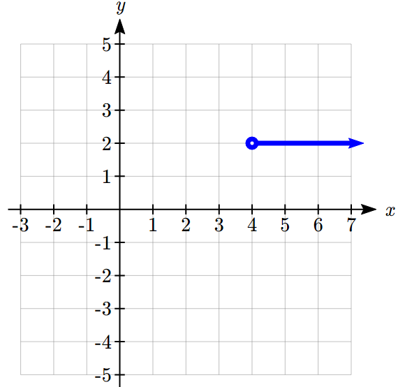
![]()
Example 7.1 H: Graphs of Functions
Which of these graphs defines a function ?

Solution:
Looking at the three graphs above, the first two define a function , since for each input value along the horizontal axis there is exactly one output value corresponding, determined by the -value of the graph. The 3rd graph does not define a function since some input values, such as  , correspond with more than one output value.
Vertical Line Test
The vertical line test is a handy way to think about whether a graph defines the vertical output as a function of the horizontal input. Imagine drawing vertical lines through the graph. If any vertical line would cross the graph more than once, then the graph does not define only one vertical output for each horizontal input.
Evaluating a function using a graph requires taking the given input and using the graph to look up the corresponding output. Solving a function equation using a graph requires taking the given output and looking on the graph to determine the corresponding input.
Example 7.1 I: Solving Functions from Graphs
Given the graph shown below,
a) Evaluate 
b) Solve 
Solution:
a) To evaluate , we find the input of on the horizontal axis. Moving up to the graph gives the point  , giving an output of
  . So
. So 
b) To solve , we find the value 4 on the vertical axis because if then 4 is the output. Moving horizontally across the graph gives two points with the output of 4:  and
and  . These give the two solutions to :
  or
or  .
.
This means  and
and  , or when the input is -1 or 3, the output is 4.
You try…
5. Using the graph from Example 7.1I, solve f(x)=1.
Formulas as Functions
When possible, it is very convenient to define relationships using formulas. If it is possible to express the output as a formula involving the input quantity, then we can define a function.
Example 7.1 J: Relationships as Functions
Express the relationship  as a function
  if possible.
Solution:
To express the relationship in this form, we need to be able to write the relationship where  is a function of , which means writing it as = [something involving ].
subtract  from both sides

divide both sides by 6 and simplify

Having rewritten the formula as  , we can now express p as a function:

It is important to note that not every relationship can be expressed as a function with a formula.
Note the important feature of an equation written as a function is that the output value can be determined directly from the input by doing evaluations – no further solving is required. This allows the relationship to act as a magic box that takes an input, processes it, and returns an output. Modern technology and computers rely on these functional relationships, since the evaluation of the function can be programmed into machines, whereas solving things is much more challenging.
As with tables and graphs, it is common to evaluate and solve functions involving formulas. Evaluating will require replacing the input variable in the formula with the value provided and calculating. Solving will require replacing the output variable in the formula with the value provided, and solving for the input(s) that would produce that output.
Example 7.1 K: Evaluating Functions
Given the function 
a) Evaluate 
b) Solve 
Solution:
a) To evaluate , we plug in the input value 2 into the formula wherever we see the input variable  , then simplify


So 
b) To solve , we set the formula for  equal to 1, and solve for the input value that will produce that output
substitute the original formula

subtract 2 from each side

take the cube root of each side

When solving an equation using formulas, you can check your answer by using your solution in the original equation to see if your calculated answer is correct.
We want to know if is true when .


which was the desired result.
Example 7.1 L: Evaluating Functions
Given the function 
a) Evaluate 
b) Solve 
Solution:
a) To evaluate we substitute the value 4 for the input variable in the given function.


b)
Substitute the original function :

This is quadratic, so we can rearrange the equation to get it = 0:

subtract 3 from each side:
this is factorable, so we factor it:

By the zero factor theorem since , either  or
or  (or both of them equal 0) and so we solve both equations for , finding
  from the first equation and
  from the second equation.
This gives us the solution: when or
You try…
6. Given the function 
a. Evaluate 
b. Solve 
You try… Answers
- Yes
- No
- Yes, it’s a function

 or
or 
- a.

b.
Section 7.1 Exercises
- Given a specific person, is their height a function of their age? Is the person’s age a function of their height? Justify your answers.
- At a coffee shop, the menu consists of items and their prices. Is price a function of the item? Is the item a function of the price? Justify your answers.
- At Ontario Tech University, the final grade a student earns in the course corresponds to a letter grade (see Ontario Tech – Grading). Is the letter grade a function of the percentage a student can obtain in the course? Is the percentage a student can obtain in the course a function of the letter grade? Justify.
- Consider bank account information.
- Is the account balance a function of the bank account number? Justify.
- Is the bank account number a function of the account balance? Justify.
- Introduce function notation of your choice using variable names to represent a function that takes as input the name of a month, and gives as output the number of days in that month. State clearly what each variable represents.
- A function
 gives the number of police officers, , in a town in year . What does
  tell us?
 - Which of these tables define a function (if any)? Justify.
-
Input Output 2 1 5 3 8 6 -
Input Output -3 5 0 1 4 5 -
Input Output 1 0 5 2 5 4
-
- Using the table shown for
 :
:
1 2 3 4 5 8 6 7 6 8 - Evaluate
 and interpret your result (describe in words what the answer means).
 - Solve
 and interpret your result.
 - Evaluate
 . Interpret your result.
 - Solve
 . Interpret your result.
- Evaluate
- Which of these graphs defines a function? Justify your answers.
- Given the graph shown,
- Evaluate .
- Solve
 .
. - Evaluate
 .
. - Solve
 .
.
- Evaluate
- If possible, express the relationship
 as a function
  .
. - Consider the relationship
 . Use this relationship to express the following functions, if possible. If this is not possible, justify why not.
- Express as a function of .
- Express as a function of .
- Express
- Given the function .
- Evaluate .
- Solve
 .
.
- Evaluate
- Given the function ,
- Evaluate .
- Solve .
- Evaluate
- Given the function
- Evaluate
- Solve
- Evaluate
7.2: Domain and Range
One of our main goals in mathematics is to model the real world with mathematical functions. In doing so, it is important to keep in mind the limitations of those models we create.
This table shows a relationship between circumference and height of a tree as it grows.
Circumference,  |
1.7 | 2.5 | 5.5 | 8.2 | 13.7 |
| Height, |
24.5 | 31 | 45.2 | 54.6 | 92.1 |
While there is a strong relationship between the two, it would certainly be ridiculous to talk about a tree with a circumference of -3 feet, or a height of 3000 feet. When we identify limitations on the inputs and outputs of a function, we are determining the domain and range of the function.
Domain and Range
The domain refers to the set of possible input values to a function.
The range refers to the set of possible output values of a function
Example 7.2 A: Domain and Range
Using the tree table above, determine a reasonable domain and range.
Solution:
We could combine the data provided with our own experiences and reason to approximate the domain and range of the function  . For the domain, possible values for the input circumference , it doesn’t make sense to have negative values, so
  . We could make an educated guess at a maximum reasonable value, or look up that the maximum circumference measured is about 119 feet[1]. With this information we would say a reasonable domain is
  feet.
feet.
Similarly for the range, it doesn’t make sense to have negative heights, and the maximum height of a tree could be looked up to be 379 feet, so a reasonable range is  feet.
feet.
Example 7.2 B: Calculating Postage
When sending a letter through the United States Postal Service, the price depends upon the weight of the letter[2], as shown in the table below. Determine the domain and range.
Letters
| Weight not Over | Price |
| 1 ounce | $0.44 |
| 2 ounces | $0.61 |
| 3 ounces | $0.78 |
| 4 ounces | $0.95 |
Solution:
Suppose we denote weight of a letter by  and price by , we can think of price is a function of weight, . We then have that
  represents the price of mailing the letter of weight .
Since acceptable weights are 3.5 ounces or less, and negative weights and weight of zero don’t make sense, the domain would be  or, in interval form,
 ![(0,3.55]](https://ecampusontario.pressbooks.pub/app/uploads/quicklatex/quicklatex.com-18a5c15bff6867f8eb2ef5795fb0e231_l3.png "Rendered by QuickLaTeX.com") .
.
Since possible prices are from a limited set of values, we can only define the range of this function by listing the possible values. We use the {…} brackets to denote the type of set made a from a list of values. Thus the range is = {$0.44, $0.61, $0.78, $0.95}.
1. The population of a small town in the year 1960 was 100 people. Since then, the population has grown to 1400 people reported during the 2010 census. Choose descriptive variables for your input and output and use interval notation to write the domain and range.
Notation
In the previous examples, we used inequalities to describe the domain and range of the functions. This is one way to describe intervals of input and output values, but is not the only way. Let us take a moment to discuss notation for domain and range.
Using inequalities, such as  , , and imply that we are interested in all values between the low and high values, including the high values in these examples.
However, occasionally we are interested in a specific list of numbers like the range for the price to send letters, = $0.44, $0.61, $0.78, or $0.95. These numbers represent a set of specific values: {0.44, 0.61, 0.78, 0.95}
Representing values as a set, or giving instructions on how a set is built, leads us to another type of notation to describe the domain and range.
Suppose we want to describe the values for a variable that are 10 or greater, but less than 30. In inequalities, we would write  .
.
When describing domains and ranges, we sometimes extend this into set notation, which would look like this:  . The curly brackets {} are read as “the set of”, and the vertical bar | is read as “such that”, so altogether we would read as “the set of -values such that 10 is less than or equal to and is less than 30.”
When describing ranges in set notation, we could similarly write something like  , or if the output had its own variable, we could use it. So for our tree height example above, we could write for the range
  . In set notation, if a domain or range is not limited, we could write {| is a real number}, or
  , read as “the set of -values such that is an element of the set of real numbers.”
A more compact alternative to set notation is interval notation, in which intervals of values are referred to by the starting and ending values. Curved parentheses are used for “strictly less than,” and square brackets are used for “less than or equal to.” Since infinity is not a number, we can’t include it in the interval, so we always use curved parentheses with  and
and  . The table below will help you see how inequalities correspond to set notation and interval notation:
| Inequality | Set Notation | Interval Notation |
 |
 |
![(5, 10]](https://ecampusontario.pressbooks.pub/app/uploads/quicklatex/quicklatex.com-0c803c4ccff68834f3858e199dd1a885_l3.png "Rendered by QuickLaTeX.com") |
 |
 |
 |
 |
 |
 |
 |
 |
 |
 |
 |
 |
| all real numbers |  |
 |
To combine two intervals together, using inequalities or set notation we can use the word “or”. In interval notation, we use the union symbol,  , to combine two unconnected intervals together.
Example 7.2 C: Intervals
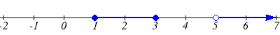
Describe the intervals of values shown on the line graph below using set builder and interval notations.
Solution:
To describe the values, , that lie in the intervals shown above we would say, “ is a real number greater than or equal to 1 and less than or equal to 3, or a real number greater than 5.”
As an inequality it is:
 or
or 
In set notation:
 or
or 
In interval notation:
![[1, 3]\cup(5, \infty)](https://ecampusontario.pressbooks.pub/app/uploads/quicklatex/quicklatex.com-8c223c1182539ec38cc5907f3b0c44e0_l3.png "Rendered by QuickLaTeX.com")
Remember when writing or reading interval notation:
- Using a square bracket [ means the start value is included in the set.
- Using a parenthesis ( means the start value is not included in the set.
2. Given the following interval, write its meaning in words, set builder notation, and interval notation.
Domain and Range from Graphs
We can also talk about domain and range based on graphs. Since domain refers to the set of possible input values, the domain of a graph consists of all the input values shown on the graph. Remember that input values are almost always shown along the horizontal axis of the graph. Likewise, since range is the set of possible output values, the range of a graph we can see from the possible values along the vertical axis of the graph.
Be careful – if the graph continues beyond the window on which we can see the graph, the domain and range might be larger than the values we can see.
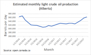
Example 7.2 D: Domain and Range of a Graph
Determine the domain and range of the graph below.
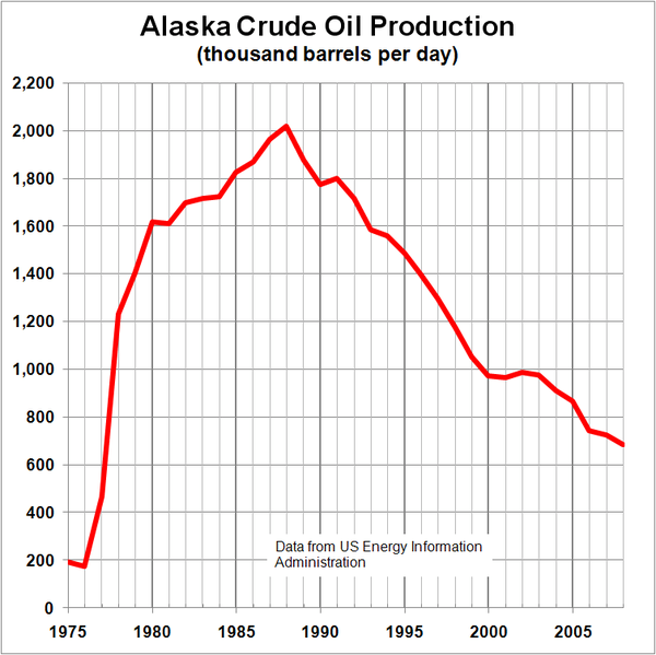
Solution:
In the graph above[3], the input quantity along the horizontal axis appears to be “year”, which we could denote by the variable . The output is “thousands of barrels of oil per day”, which we might denote by the variable  , for barrels. The graph would likely continue to the left and right beyond what is shown, but based on the portion of the graph that is shown to us, we can determine the domain is
  , and the range is approximately
  .
.
In interval notation, the domain would be ![[1975, 2008]](https://ecampusontario.pressbooks.pub/app/uploads/quicklatex/quicklatex.com-541c3d214a17d8f44d2dbae1e78d8161_l3.png "Rendered by QuickLaTeX.com") and the range would be about
and the range would be about ![[180, 2010]](https://ecampusontario.pressbooks.pub/app/uploads/quicklatex/quicklatex.com-dda5a4172bddc1a209cd11e65f9474ea_l3.png "Rendered by QuickLaTeX.com") . For the range, we have to approximate the smallest and largest outputs since they don’t fall exactly on the grid lines.
. For the range, we have to approximate the smallest and largest outputs since they don’t fall exactly on the grid lines.
Remember that, as in the previous example, and are not always the input and output variables. Using descriptive variables is an important tool to remembering the context of the problem.
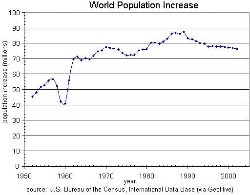
You try…
3. Given the graph below, write the domain and range in interval notation.
Domain and Range from Formulas
Most basic formulas can be evaluated at an input. Two common restrictions are:
- The square root of negative values is non-real.
- We cannot divide by zero.
Example 7.2 E: Finding Domain and Range
Find the domain of each function:
a) 
b) 
Solution:
a) Since we cannot take the square root of a negative number, we need the inside of the square root to be non-negative.
 when
when  .
.
The domain of  is
is  .
.
b) We cannot divide by zero, so we need the denominator to be non-zero.
 when ,
so we must exclude 2 from the domain.
The domain of  is
is  .
.
Piecewise Functions
Some functions cannot be described by a single formula.
Piecewise Function
A piecewise function is a function in which the formula used depends upon the domain the input lies in. We notate this idea like:

Example 7.2 F: Piecewise Functions
A museum charges $5 per person for a guided tour with a group of 1 to 9 people, or a fixed $50 fee for 10 or more people in the group. Set up a function relating the number of people, , to the cost,  .
.
Solution:
To set up this function, two different formulas would be needed.  would work for values under 10, and
  would work for values of ten or greater. We denote this as follows:

Example 7.2 G: Applications of Piecewise Functions
A cell phone company uses the function below to determine the cost, , in dollars for gigabytes of data transfer.

Find the cost of using 1.5 gigabytes of data, and the cost of using 4 gigabytes of data.
Solution:
To find the cost of using 1.5 gigabytes of data,  , we first look to see which piece of domain our input falls in. Since 1.5 is less than 2, we use the first formula, giving
  .
.
To find the cost of using 4 gigabytes of data,  , we see that our input of 4 is greater than 2, so we’ll use the second formula.
  .
.
Therefore, the cost of using 1.5 gigabytes of data is $25, and the cost of using 4 gigabytes of data is $45.
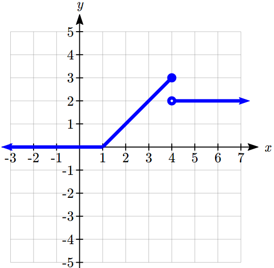
Example 7.2 H: Graphing a Piecewise Function
Sketch a graph of the function

Solution:
We can imagine graphing each function, then limiting the graph to the indicated domain. At the endpoints of the domain, we put open circles to indicate where the endpoint is not included, due to a strictly-less-than inequality, and a closed circle where the endpoint is included, due to a less-than-or-equal-to inequality. The first and last parts are constant functions, where the output is the same for all inputs. The middle part we might recognize as a line, and could graph by evaluating the function at a couple inputs and connecting the points with a line.
Now that we have each piece individually, we combine them onto the same graph. When the first and second parts meet at  , we can imagine the closed dot filling in the open dot. Since there is no break in the graph, there is no need to show the dot.
You try…
4. At Pierce College during the 2009-2010 school year tuition rates for in-state residents were $89.50 per credit for the first 10 credits, $33 per credit for credits 11-18, and for over 18 credits the rate is $73 per credit[4].
Write a piecewise defined function for the total tuition,  , at Pierce College during 2009-2010 as a function of the number of credits taken, . Be sure to consider a reasonable domain and range.
You try… Answers
1. Domain: = years ![[1960, 2010]](https://ecampusontario.pressbooks.pub/app/uploads/quicklatex/quicklatex.com-3147877397be38dd4c48f268281f0417_l3.png "Rendered by QuickLaTeX.com")
Range: = population, ![[100, 1400]](https://ecampusontario.pressbooks.pub/app/uploads/quicklatex/quicklatex.com-77ddb6b39db24a6233f7f070daf87659_l3.png "Rendered by QuickLaTeX.com")
2. a. Values that are less than or equal to -2, or values that are greater than or equal to -1 and less than 3
b. 
c. ![( - \infty , - 2] \cup [ - 1,3)](https://ecampusontario.pressbooks.pub/app/uploads/quicklatex/quicklatex.com-f7ad7f9594afaf97a1e99777f3c9deb1_l3.png "Rendered by QuickLaTeX.com")
3. Domain: =years ![[1952, 2002]](https://ecampusontario.pressbooks.pub/app/uploads/quicklatex/quicklatex.com-515d48c1bb657d3a7d27ab2e645daf6a_l3.png "Rendered by QuickLaTeX.com")
Range: =population in millions, ![[40, 88]](https://ecampusontario.pressbooks.pub/app/uploads/quicklatex/quicklatex.com-b5ace8bf65bdee10e6f850801e20b0c2_l3.png "Rendered by QuickLaTeX.com")
4. Tuition, , as a function of credits, .

Reasonable domain should be whole numbers 0 to (answers may vary), e.g. ![[0, 23]](https://ecampusontario.pressbooks.pub/app/uploads/quicklatex/quicklatex.com-a093be9c18f52c3e97f9f5e4368e4287_l3.png "Rendered by QuickLaTeX.com")
Reasonable range should be $0 – (answers may vary), e.g. ![[0, 1524]](https://ecampusontario.pressbooks.pub/app/uploads/quicklatex/quicklatex.com-0d84e0bbf844db6e7c08fc0637e2164b_l3.png "Rendered by QuickLaTeX.com")
Section 7.2 Exercises
- A data storage company rents server space for a flat annual fee of $150 and storage charge of $0.39 per GB for less than 1.8 petabytes per annual contract (one petabyte is 1000 terabytes and one terabyte is 1000 GB).
- Write the formula for the total cost to rent server space as a function of the
 gigabytes of data storage requirement.
 - What is the domain of this function?
- What is the range of this function?
- Find the total cost to rent server space for 3.5 terabytes of storage space.
- Determine how much server space was rented under the annual contract if the bill was $1203.
- Write the formula for the total cost
- A rental car company rents cars for a flat fee of $20 and an hourly charge of $10.25. Reservations made but cancelled are charged the flat fee. The company policy states that the rentals must be less than 5 days in duration.
- Write the formula for the total cost to rent a car as a function of the hours the car is rented.
- What is the domain of this function?
- What is the range of this function?
- Find the total cost to rent a car for 2 days and 7 hours.
- Write the formula for the total cost
- In making strategic decisions in manufacturing we study the relationship between market supply of an item and the price of the item. Suppose the number of units available at the price of the unit of a particular product satisfy the following relationship:

- If possible, express the supply as a function of the price, explain what that means and why it is useful. If it is not possible, explain why.
- If possible, express the price as a function of the supply, explain what that means and why it is useful. If it is not possible, explain why.
- What is the domain of the supply function in terms of price?
- In making strategic decisions about product pricing, we study the relationship between market demand for an item and the price of the item. Suppose the market demand for number of units and the price of the unit of a particular product satisfy the following relationship:

- If possible, express the demand as a function of price, explain what that means and why it is useful. If it is not possible, explain why.
- If possible, express the price as a function of demand, explain what that means and why it is useful. If it is not possible, explain why.
- What is the domain of the demand function in terms of price?
- What is the domain of the price function in terms of demand?
- If the revenues from sales of units of a certain product and the cost of manufacturing units of the same product can be expressed as
 and
and  ,
,
- Determine the profit function in terms of the number of units .
- Calculate and interpret what that means.
- Calculate and interpret what that means.
- How many units would they have to produce and sell to break even?
- The population of Oshawa in the year 1960 was 77,000 people. Since then the population has grown to 379,848 people reported during the 2016 census. Choose descriptive variables for your input and output and use interval notation to write the domain and range.
- Describe the domains of
- A phone data plan has a basic charge of $30 a month. The plan includes first 2GB free and charges $10 for each additional GB, up to 8 GB total usage, after which it charges $15 for each additional GB. If is the amount of data used (in GB) and is the total monthly cost:
- Express
 as a (piece-wise) formula.
 - Identify the independent and the dependent variables of C.
- Identify the domain and the range of .
- Graph as a function of for
 .
. - Calculate the cost if 9GB were used.
- Express
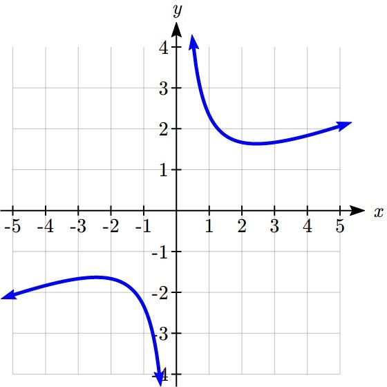
- Describe the relationship shown in the graph below as a function and describe its domain and range in interval form.
- Population Growth: The table below lists the Canada population by census years (source: Statistics Canada).
Census Year Canadian Population (millions) 1991 27.3 1996 28.8 2001 30.0 2006 31.5 2011 33.5 2016 35.2 - Using Microsoft Excel, find a linear regression model that represents the size of Canadian population in millions in terms of number of years since 1991 and graph the model.
- Draw a scatter plot of the data and graph the model.
- Interpret the slope of the model.
- Estimate the size of Canadian population in 2003.
- Predict the population of Canada in 2030.


![f(x)=\frac{x}{\sqrt[3]{x+3}}](https://ecampusontario.pressbooks.pub/app/uploads/quicklatex/quicklatex.com-306de096a2a8857253823e289a70e539_l3.png "Rendered by QuickLaTeX.com")
7.3: Rates of Change and Behaviour of Graphs
Since functions represent how an output quantity varies with an input quantity, it is natural to ask about the rate at which the values of the function are changing.
For example, the function  below gives the average cost, in dollars, of a gallon of gasoline years after 2000.
|
2 | 3 | 4 | 5 | 6 | 7 | 8 | 9 |
|
1.47 | 1.69 | 1.94 | 2.30 | 2.51 | 2.64 | 3.01 | 2.14 |
If we were interested in how the gas prices had changed between 2002 and 2009, we could compute that the cost per gallon had increased from $1.47 to $2.14, an increase of $0.67. While this is interesting, it might be more useful to look at how much the price changed per year. You are probably noticing that the price didn’t change the same amount each year, so we would be finding the average rate of change over a specified amount of time.
The gas price increased by $0.67 from 2002 to 2009, over 7 years, for an average of  dollars per year.
On average, the price of gas increased by about 9.6 cents each year.
Rate of Change
A rate of change describes how the output quantity changes in relation to the input quantity. The units on a rate of change are “output units per input units”
Some other examples of rates of change would be quantities like:
- A population of rats increases by 40 rats per week
- A barista earns $9 per hour (dollars per hour)
- A farmer plants 60,000 onions per acre
- A car can drive 27 miles per gallon
- A population of grey whales decreases by 8 whales per year
- The amount of money in your college account decreases by $4,000 per quarter
Average Rate of Change
The average rate of change between two input values is the total change of the function values (output values) divided by the change in the input values.
Average rate of change =  =
= 
Example 7.3 A: Cost Functions
Using the cost-of-gas function from earlier, find the average rate of change between 2007 and 2009.
From the table, in 2007 the cost of gas was $2.64. In 2009 the cost was $2.14.
The input (years) has changed by 2. The output has changed by $2.14 – $2.64 = -0.50.
The average rate of change is then  dollars per year
1. Using the same cost-of-gas function, find the average rate of change between 2003 and 2008
Notice that in the last example the change of output was negative since the output value of the function had decreased. Correspondingly, the average rate of change is negative.
Example 7.3 B: Average Rate of Change
Given the function  shown here, find the average rate of change on the interval
 ![[0, 3]](https://ecampusontario.pressbooks.pub/app/uploads/quicklatex/quicklatex.com-8904eed563010edb5b7669e987a306c7_l3.png "Rendered by QuickLaTeX.com") .
.
At  , the graph shows
At  , the graph shows
The output has changed by 3 while the input has changed by 3, giving an average rate of change of:

Example 7.3 C: Average Speed
On a road trip, after picking up your friend who lives 10 miles away, you decide to record your distance from home over time. Find your average speed over the first 6 hours.
| (hours) |
0 | 1 | 2 | 3 | 4 | 5 | 6 | 7 |
 (miles) (miles) |
10 | 55 | 90 | 153 | 214 | 240 | 292 | 300 |
Here, your average speed is the average rate of change.
You traveled 282 miles in 6 hours, for an average speed of  = 47 miles per hour
We can more formally state the average rate of change calculation using function notation.
Average Rate of Change using Function Notation
Given a function , the average rate of change on the interval ![[a, b]](https://ecampusontario.pressbooks.pub/app/uploads/quicklatex/quicklatex.com-93a1866e932ce9856cd5794c5591a6cd_l3.png "Rendered by QuickLaTeX.com") is
is
Average rate of change = 
Example 7.3 D: Average Rate of Change
Compute the average rate of change of  on the interval
 ![[2, 4]](https://ecampusontario.pressbooks.pub/app/uploads/quicklatex/quicklatex.com-00853d4bf1c3f16806315114fada7d73_l3.png "Rendered by QuickLaTeX.com") .
.
We can start by computing the function values at each endpoint of the interval


Now computing the average rate of change
Average rate of change = 
2. Find the average rate of change of  on the interval
 ![[1, 9]](https://ecampusontario.pressbooks.pub/app/uploads/quicklatex/quicklatex.com-afe80f85e606f4b62af906b6c0cf3f18_l3.png "Rendered by QuickLaTeX.com") .
.
Example 7.3 E: Magnetic Force
The magnetic force  , measured in Newtons, between two magnets is related to the distance between the magnets , in centimeters, by the formula
  . Find the average rate of change of force if the distance between the magnets is increased from 2 cm to 6 cm.
We are computing the average rate of change of on the interval ![[2, 6]](https://ecampusontario.pressbooks.pub/app/uploads/quicklatex/quicklatex.com-10359ab7cf2b96e16fa1e1b239665851_l3.png "Rendered by QuickLaTeX.com") .
.
Average rate of change = 
Evaluating the function

Simplifying

Combining the numerator terms

Simplifying further
 Newtons per centimeter
This tells us the magnetic force decreases, on average, by  Newtons per centimeter over this interval.
Example 7.3 F: Average Rate of Change
Find the average rate of change of  on the interval
 ![[0, a]](https://ecampusontario.pressbooks.pub/app/uploads/quicklatex/quicklatex.com-2e19a55961d16dde8b8bac3a63a51dd4_l3.png "Rendered by QuickLaTeX.com") . Your answer will be an expression involving .
. Your answer will be an expression involving .
Using the average rate of change formula

Evaluating the function

Simplifying

Simplifying further, and factoring

Cancelling the common factor

This result tells us the average rate of change between and any other point  . For example, on the interval
 ![[0, 5]](https://ecampusontario.pressbooks.pub/app/uploads/quicklatex/quicklatex.com-f62215b0478e0621f8df62dfef473cfb_l3.png "Rendered by QuickLaTeX.com") , the average rate of change would be 5+3 = 8.
, the average rate of change would be 5+3 = 8.
3. Find the average rate of change of  on the interval
 ![[a, a + h]](https://ecampusontario.pressbooks.pub/app/uploads/quicklatex/quicklatex.com-238923f464e7a574c55502194abc304b_l3.png "Rendered by QuickLaTeX.com") .
.
Application to Business
In business, average rate of change is related to the idea of marginal cost, marginal revenue, and marginal profit.
Marginal Cost/Revenue/Profit
Marginal Cost is typically defined as the change in total cost if the quantity of items produced increases by one. Likewise, marginal revenue and marginal profit are the change in revenue and profit if the quantity of items increases by one.
In practice, marginal cost is usually calculated another way, using calculus techniques you will learn in future courses. In this course, though, we will stick with calculating marginal cost by looking at the actual change of total cost when production increases by one.
Example 7.3 G: Marginal Cost
A company has determined the total cost of producing  items is
  . Find the marginal cost, when production is currently 5000 items.
We want to find the increase in total cost when increasing production from 5000 items to 5001 items. This is equivalent to finding the average rate of change on the interval ![[5000, 5001]](https://ecampusontario.pressbooks.pub/app/uploads/quicklatex/quicklatex.com-8310dcf2528bd86806d46b400ea13279_l3.png "Rendered by QuickLaTeX.com") .
.
The total cost at 5000 items is:

The total cost at 5001 items is:

The marginal cost is
5535.89 – 5535.53 = $0.36.
In other words, after producing 5000 items, the additional cost of producing the 5001st item is $0.36
Graphical Behaviour of Functions
As part of exploring how functions change, it is interesting to explore the graphical behaviour of functions.
Increasing/Decreasing
A function is increasing on an interval if the function values increase as the inputs increase. More formally, a function is increasing if  for any two input values and in the interval with
  . The average rate of change of an increasing function is positive.
A function is decreasing on an interval if the function values decrease as the inputs increase. More formally, a function is decreasing if  for any two input values and in the interval with . The average rate of change of a decreasing function is negative.
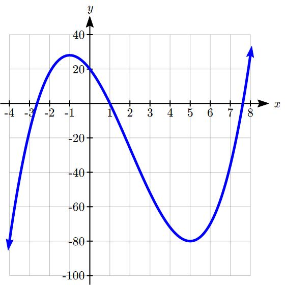
Example 7.3 H: Graphs of Functions
Given the function  graphed here, on what intervals does the function appear to be increasing?
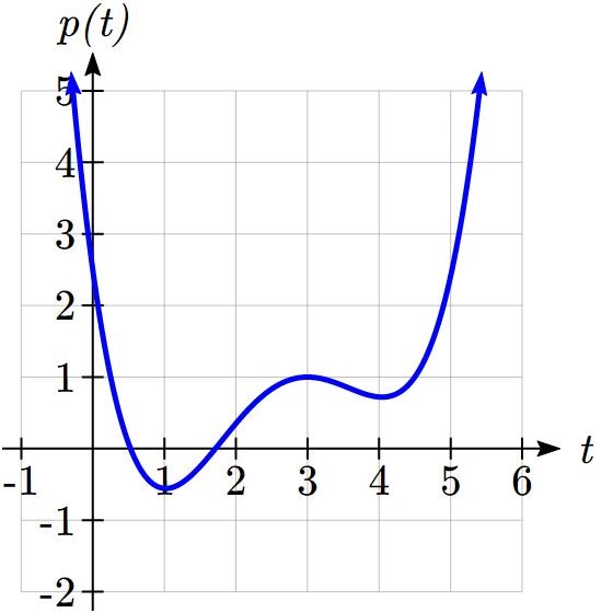
The function appears to be increasing from  to
to  , and from
  on.
on.
In interval notation, we would say the function appears to be increasing on the interval  and the interval
  .
.
Notice in the last example that we used open intervals (intervals that don’t include the endpoints) since the function is neither increasing nor decreasing at = 1, 3, or 4.
Local Extrema
A point where a function changes from increasing to decreasing is called a local maximum.
A point where a function changes from decreasing to increasing is called a local minimum.
Together, local maxima and minima are called the local extrema, or local extreme values, of the function.
Example 7.3 I: Invervals
Using the cost of gasoline function from the beginning of the section, find an interval on which the function appears to be decreasing. Estimate any local extrema using the table.
|
2 | 3 | 4 | 5 | 6 | 7 | 8 | 9 |
|
1.47 | 1.69 | 1.94 | 2.30 | 2.51 | 2.64 | 3.01 | 2.14 |
It appears that the cost of gas increased from  to
to  . It appears the cost of gas decreased from to
  , so the function appears to be decreasing on the interval
  .
.
Since the function appears to change from increasing to decreasing at , there is local maximum at .
Example 7.3 J: Estimating Extrema
Use a graph to estimate the local extrema of the function  . Use these to determine the intervals on which the function is increasing.
Using technology to graph the function, it appears there is a local minimum somewhere between and  , and a symmetric local maximum somewhere between
  and
and  .
.
Most graphing calculators and graphing utilities can estimate the location of maxima and minima. Below are screen images from two different technologies, showing the estimate for the local maximum and minimum.
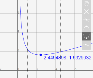
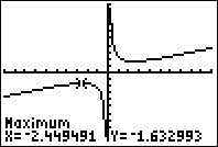
Based on these estimates, the function is increasing on the intervals  and
and  . Notice that while we expect the extrema to be symmetric, the two different technologies agree only up to 4 decimals due to the differing approximation algorithms used by each.
4. Use a graph of the function  to estimate the local extrema of the function. Use these to determine the intervals on which the function is increasing and decreasing.
Give It Some Thought Answers
1.  = 0.264 dollars per year.
2. Average rate of change = 
3. 

4. Based on the graph, the local maximum appears to occur at  , and the local minimum occurs at
  . The function is increasing on
  and decreasing on
  .
.
Section 7.3 Exercises
Insert review exercises here
7.4: Linear Functions
As you hop into a taxicab in Las Vegas, the meter will immediately read $3.30; this is the “drop” charge made when the taximeter is activated. After that initial fee, the taximeter will add $2.60 for each mile the taxi drives[5]. In this scenario, the total taxi fare depends upon the number of miles ridden in the taxi, and we can ask whether it is possible to model this type of scenario with a function. Using descriptive variables, we choose for miles and for Cost in dollars as a function of miles:  .
.
We know for certain that  , since the $3.30 drop charge is assessed regardless of how many miles are driven. Since $2.60 is added for each mile driven, then:

If we then drove a second mile, another $2.60 would be added to the cost:

If we drove a third mile, another $2.40 would be added to the cost:

From this we might observe the pattern, and conclude that if miles are driven,  because we start with a $3.30 drop fee and then for each mile increase we add $2.60.
It is good to verify that the units make sense in this equation. The $3.30 drop charge is measured in dollars; the $2.60 charge is measured in dollars per mile. So

When dollars per mile are multiplied by a number of miles, the result is a number of dollars, matching the units on the 3.30, and matching the desired units for the function.
Notice this equation consisted of two quantities. The first is the fixed $3.30 charge which does not change based on the value of the input. The second is the $2.60 dollars per mile value, which is a rate of change. In the equation this rate of change is multiplied by the input value.
Looking at this same problem in table format we can also see the cost changes by $2.60 for every 1 mile increase.
|
0 | 1 | 2 | 3 |
|
3.30 | 5.90 | 8.50 | 11.10 |
It is important here to note that in this equation, the rate of change is constant; over any interval, the rate of change is the same.
Graphing this equation, we see the shape is a line, which is how these functions get their name: linear functions.
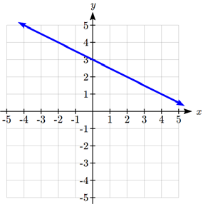
When the number of miles is zero the cost is $3.30, giving the point (0, 3.30) on the graph. This is the vertical or intercept. The graph is increasing in a straight line from left to right because for each mile the cost goes up by $2.40; this rate remains consistent.
In this example you have seen the taxicab cost modeled in words, an equation, a table and in graphical form. Whenever possible, ensure that you can link these four representations together to continually build your skills. It is important to note that you will not always be able to find all 4 representations for a problem and so being able to work with all 4 forms is very important.
Linear Function
A linear function is a function whose graph produces a line. Linear functions can always be written in the form

or

They’re equivalent where:
is the initial or starting value of the function (when input, ), and
is the constant rate of change of the function
Many people like to write linear functions in the form  because it corresponds to the way we tend to speak: “The output starts at and increases at a rate of .”
For this reason alone we will use the form for many of the examples, but remember they are equivalent and can be written correctly both ways.
Slope and Increasing/Decreasing
is the constant rate of change of the function (also called slope). The slope determines if the function is an increasing function or a decreasing function.
is an increasing function if 
is a decreasing function if 
If  , the rate of change zero, and the function
  is just a horizontal line passing through the point
  , neither increasing nor decreasing.
Example 7.4A
To start producing a new model of custom wheels, a company will have to purchase $30,000 in new equipment. Each wheel made costs them $40 in supplies and labor. Write a formula for the total cost,  , of producing wheels. What will be their total costs in the first year if they expect to sell 240 wheels?
The initial value for this function is 30,000, since that is the startup costs, so
 . The cost increases by $40 for each wheel made, so the rate of change is $40 per wheel. With this information, we can write the formula:
.
 is an increasing linear function.
With this formula we can predict the total cost of 240 wheels:
 .
.
The total cost will be $39,600.
1. If you earn $30,000 per year and you spend $29,000 per year write an equation for the amount of money you save after years, if you start with nothing.
“The most important thing, spend less than you earn!”[6]
Calculating Rate of Change
Given two values for the input,  and
and  , and two corresponding values for the output,
  and
and  , or a set of points,
  and
and  , if we wish to find a linear function that contains both points we can calculate the rate of change, :

Rate of change of a linear function is also called the slope of the line.
Note in function notation,  and
and  , so we could equivalently write

Example 7.4B
The population of a city increased from 23,400 to 27,800 between 2002 and 2006. Find the rate of change of the population during this time span.
The rate of change will relate the change in population to the change in time. The population increased by  people over the 4 year time interval. To find the rate of change, the number of people per year the population changed by:
 = 1100 people per year
Notice that we knew the population was increasing, so we would expect our value for m to be positive. This is a quick way to check to see if your value is reasonable.
Example 7.4C
The pressure,  , in pounds per square inch (PSI) on a diver depends upon their depth below the water surface, , in feet, following the equation
  . Interpret the components of this function.
The rate of change, or slope, 0.434 would have units
 .
.
This tells us the pressure on the diver increases by 0.434 PSI for each foot their depth increases.
The initial value, 14.696, will have the same units as the output, so this tells us that at a depth of 0 feet, the pressure on the diver will be 14.696 PSI.
Example 7.4D
If is a linear function,  , and
, and  , find the rate of change.
tells us that the input 3 corresponds with the output -2, and tells us that the input 8 corresponds with the output 1. To find the rate of change, we divide the change in output by the change in input:
 .
.
If desired we could also write this as  .
.
Note that it is not important which pair of values comes first in the subtractions so long as the first output value used corresponds with the first input value used.
2. Given the two points  and
and  , find the rate of change. Is this function increasing or decreasing?
We can now find the rate of change given two input-output pairs, and can write an equation for a linear function once we have the rate of change and initial value. If we have two input-output pairs and they do not include the initial value of the function, then we will have to solve for it.
Example 7.4E
Write an equation for the linear function graphed below.
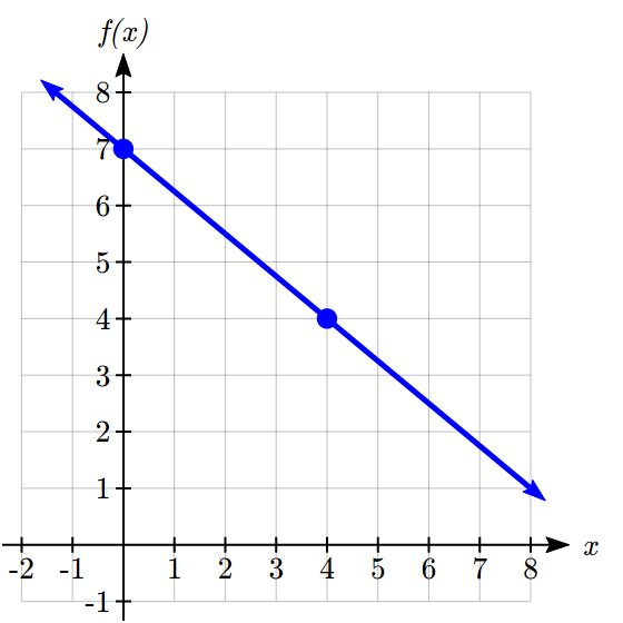
Looking at the graph, we might notice that it passes through the points  and
and  . From the first value, we know the initial value of the function is
  , so in this case we will only need to calculate the rate of change:

This allows us to write the equation:

Example 7.4F
If is a linear function, , and , find an equation for the function.
In Example 7.4C, we computed the rate of change to be  . In this case, we do not know the initial value
  , so we will have to solve for it. Using the rate of change, we know the equation will have the form
  . Since we know the value of the function when , we can evaluate the function at 3.

Since we know that , we can substitute on the left side

This leaves us with an equation we can solve for the initial value

Combining this with the value for the rate of change, we can now write a formula for this function:

Example 7.4G
Working as an insurance salesperson, Ilya earns a base salary and a commission on each new policy, so Ilya’s weekly income,  , depends on the number of new policies, , he sells during the week. Last week he sold 3 new policies, and earned $760 for the week. The week before, he sold 5 new policies, and earned $920. Find an equation for
  , and interpret the meaning of the components of the equation.
The given information gives us two input-output pairs:  and
and  . We start by finding the rate of change.

Keeping track of units can help us interpret this quantity. Income increased by $160 when the number of policies increased by 2, so the rate of change is $80 per policy; Ilya earns a commission of $80 for each policy sold during the week.
We can then solve for the initial value

then when  ,
,  , giving

this allows us to solve for

This value is the starting value for the function. This is Ilya’s income when  , which means no new policies are sold. We can interpret this as Ilya’s base salary for the week, which does not depend upon the number of policies sold.
Writing the final equation:

Our final interpretation is: Ilya’s base salary is $520 per week and he earns an additional $80 commission for each policy sold each week.
3. Looking at Example 7.4G:
Determine the independent and dependent variables.
What is a reasonable domain and range?
4.The balance in your college payment account, , is a function of the number of quarters, , you attend. Interpret the function  in words. How many quarters of college can you pay for until this account is empty?
Example 7.4H
Given the table below write a linear equation that represents the table values
| , number of weeks |
0 | 2 | 3 | 6 |
 , number of rats , number of rats |
1000 | 1080 | 1160 | 1240 |
We can see from the table that the initial value of rats is 1000 so in the linear format  ,
,  .
.
Rather than solving for , we can notice from the table that the population goes up by 80 for every 2 weeks that pass. This rate is consistent from week 0, to week 2, 4, and 6. The rate of change is 80 rats per 2 weeks. This can be simplified to 40 rats per week and we can write
as

If you didn’t notice this from the table you could still solve for the slope using any two points from the table. For example, using  and
and  ,
,
 rats per week
Give It Some Thought Answers
1.  $1000 is saved each year.
2.  ; Decreasing because
3. (number of policies sold) is the independent variable
(weekly income as a function of policies sold) is the dependent variable.
A reasonable domain is  *
*
A reasonable range is  *
*
*answers may vary given reasoning is stated; 15 is an arbitrary upper limit based on selling 3 policies per day in a 5 day work week and $1740 corresponds with the domain.
4. Your College account starts with $20,000 in it and you withdraw $4,000 each quarter (or your account contains $20,000 and decreases by $4000 each quarter.) You can pay for 5 quarters before the money in this account is gone.
Section 7.4 Exercises
- Sarah wants to go skating at Super Skate ice rink. She has to pay a $7 entrance fee and $1.25 for every minute she is on the rink.
- Write an equation to determine the cost (C) in terms of the number of minutes (t) that she is on the rink.
- If she only has $43.25, find the number of minutes she can be on the rink.
- If you earn $30,000 per year and you spend $29,000 per year, write amount of money you save
 after years, assuming you start with no money.
 - The balance in your post-secondary studies savings account
 , is a function of the number of terms you attend. Interpret the function in words and explain the meaning of each number and symbol in this equation. For how many terms of post-secondary education can you pay until this account is empty?
 - A manager for a country market will spend a total of $80 on apples at $0.25 each and pears at $0.50 each. Write the number of apples she can buy as a linear function of the number of pears. Find the slope and interpret your answer. Graph the function.
- At $10 per ticket, Willie Williams and the Wranglers will fill all 8,000 seats in the Assembly Center. The manager knows that for every $1 increase in the price, 500 tickets will go unsold.
- Write the number of tickets sold n as a function of the ticket price p.
- What are the limits of the independent variable, if any?
- At a price of $2.28 per bushel, the supply of barley is 7,500 million bushels and the demand is 7,900 million bushels. At a price of $2.37 per bushel, the supply is 7,900 million bushels and the demand is 7,800 bushels.
- Assuming that price and supply are linearly related, determine the price in terms of supply (the price-supply equation).
- Assuming that price and demand are linearly related, determine the price in terms of demand (the price-demand equation).
- Find the equilibrium point (price and the number of units for which supply and demand are equal).
- Graph the price-supply equation, price-demand equation and the equilibrium point in the same coordinate system.
7.5: Graphs of Linear Functions
When we are working with a new function, it is useful to know as much as we can about the function: its graph, where the function is zero, and any other special behaviours of the function.
When graphing a linear function, there are two basic ways to graph it:
- By plotting points (at least 2) and drawing a line through the points
- Using the initial value (output when x = 0) and rate of change (slope)
Example 7.5A
Graph  by plotting points
In general, we evaluate the function at two or more inputs to find at least two points on the graph. Usually it is best to pick input values that will “work nicely” in the equation. In this equation, multiples of 3 will work nicely due to the  in the equation, and of course using to get the vertical intercept. Evaluating at = 0, 3 and 6:

These evaluations tell us that the points  ,
,  , and
, and  lie on the graph of the line. Plotting these points and drawing a line through them gives us the graph.
When using the initial value and rate of change to graph, we need to consider the graphical interpretation of these values. Remember the initial value of the function is the output when the input is zero, so in the equation , the graph includes the point . On the graph, this is the vertical intercept – the point where the graph crosses the vertical axis.
For the rate of change, it is helpful to recall that we calculated this value as

From a graph of a line, this tells us that if we divide the vertical difference, or rise, of the function outputs by the horizontal difference, or run, of the inputs, we will obtain the rate of change, also called slope of the line.

Notice that this ratio is the same regardless of which two points we use
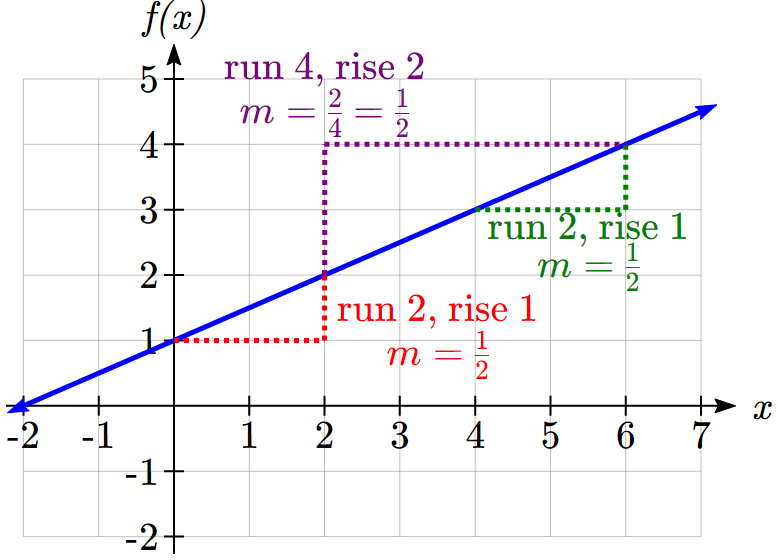
Graphical Interpretation of a Linear Equation
Graphically, in the equation
is the vertical intercept of the graph and tells us we can start our graph at
is the slope of the line and tells us how far to rise & run to get to the next point
Once we have at least 2 points, we can extend the graph of the line to the left and right.
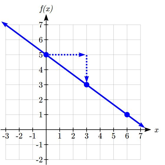
Example 7.5B
Graph using the vertical intercept and slope.
The vertical intercept of the function is , giving us a point on the graph of the line.
The slope is  . This tells us that for every 3 units the graph “runs” in the horizontal, the vertical “rise” decreases by 2 units. In graphing, we can use this by first plotting our vertical intercept on the graph, then using the slope to find a second point. From the initial value the slope tells us that if we move to the right 3, we will move down 2, moving us to the point . We can continue this again to find a third point at . Finally, extend the line to the left and right, containing these points.
1. Consider that the slope -2/3 could also be written as  . Using , find another point on the graph that has a negative value.
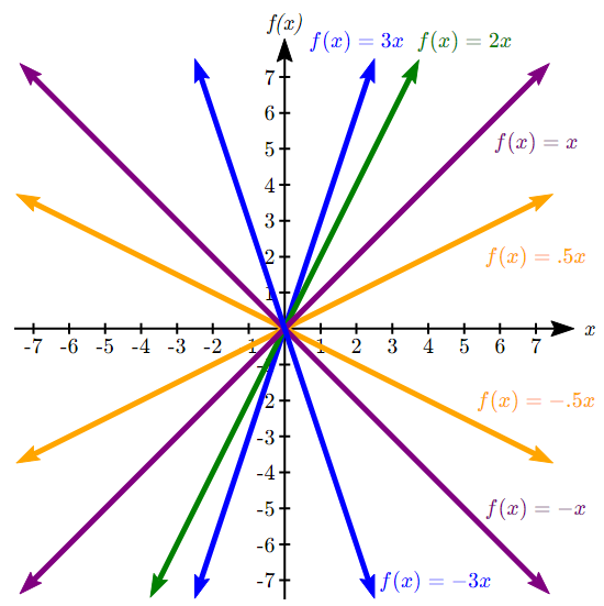
In , the value of determines the steepness of the line. When is positive the graph will be increasing, and when is negative the graph will be decreasing. Looking at some examples:
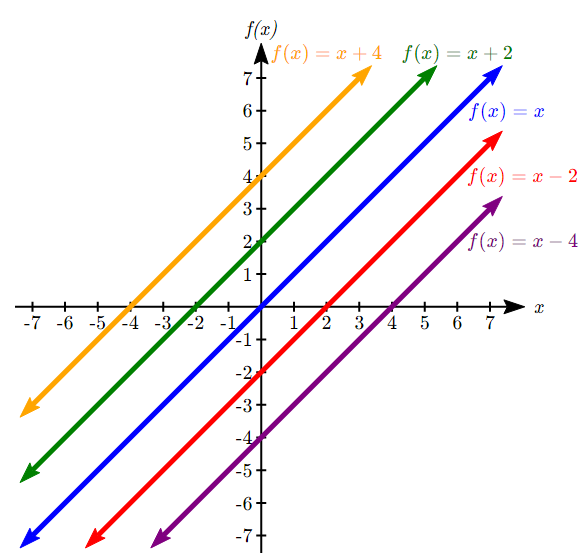
In , the acts as a vertical shift, moving the graph up and down without affecting the slope of the line. Some examples:
Example 7.5C
Match each equation with one of the lines in the graph below

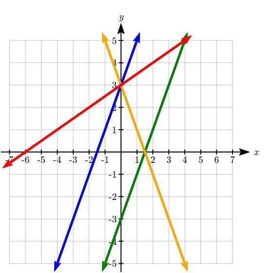
Only one graph has a vertical intercept of -3, so we can immediately match that graph with . For the three graphs with a vertical intercept at 3, only one has a negative slope, so we can match that line with  . Of the other two, the steeper line would have a larger slope, so we can match that graph with equation , and the flatter line with the equation
  .
.
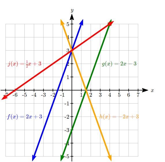
In addition to understanding the basic behaviour of a linear function (increasing or decreasing, recognizing the slope and vertical intercept), it is often helpful to know the horizontal intercept of the function – where it crosses the horizontal axis.
Finding Horizontal Intercept
The horizontal intercept of the function is where the graph crosses the horizontal axis. If a function has a horizontal intercept, you can always find it by solving  .
.
Example 7.5D
Find the horizontal intercept of  .
.
Setting the function equal to zero to find what input will put us on the horizontal axis:

The graph crosses the horizontal axis at (6,0)
There are two special cases of lines: a horizontal line and a vertical line. In a horizontal line like the one graphed below, notice that between any two points, the change in the outputs is 0. In the slope equation, the numerator will be 0, resulting in a slope of 0. Using a slope of 0 in the , the equation simplifies to 
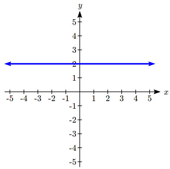
Notice a horizontal line has a vertical intercept, but no horizontal intercept (unless it’s the line ).
In the case of a vertical line, notice that between any two points, the change in the inputs is 0. In the slope equation, the denominator will be 0, and you may recall that we cannot divide by the 0; the slope of a vertical line is undefined. You might also notice that a vertical line is not a function. To write the equation of vertical line, we simply write input=value, like  .
.
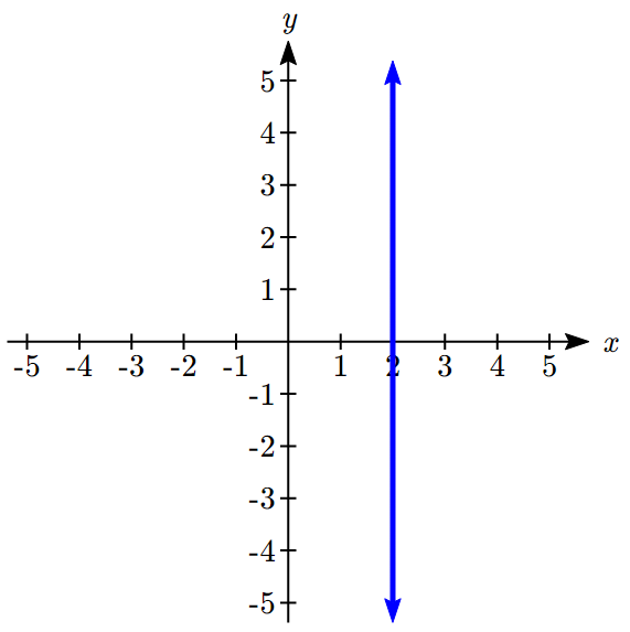
Notice a vertical line has a horizontal intercept, but no vertical intercept (unless it’s the line ).
Horizontal and Vertical Lines
Horizontal lines have equations of the form
Vertical lines have equations of the form 
Example 7.5E
Write an equation for the horizontal line graphed above.
This line would have equation 
Example 7.5F
Write an equation for the vertical line graphed above.
This line would have equation
Parallel and Perpendicular Lines
When two lines are graphed together, the lines will be parallel if they are increasing at the same rate – if the rates of change are the same. In this case, the graphs will never cross (unless they’re the same line).
Parallel Lines
Two lines are parallel if the slopes are equal (or, if both lines are vertical). In other words, given two linear equations  and
and 
The lines will be parallel if 
Example 7.5G
Find a line parallel to  that passes through the point
We know the line we’re looking for will have the same slope as the given line,  . Using this and the given point, we can solve for the new line’s vertical intercept:

then at ,

The line we’re looking for is 
If two lines are not parallel, one other interesting possibility is that the lines are perpendicular, which means the lines form a right angle (90 degree angle – a square corner) where they meet. In this case, the slopes when multiplied together will equal -1. Solving for one slope leads us to the definition:
Perpendicular Lines
Given two linear equations and
The lines will be perpendicular if  , and so
We often say the slope of a perpendicular line is the “negative reciprocal” of the other line’s slope.
Example 7.5H
Find the slope of a line perpendicular to a line with:
a) a slope of 2.
b) a slope of -4.
c) a slope of .
If the original line had slope 2, the perpendicular line’s slope would be

If the original line had slope -4, the perpendicular line’s slope would be

If the original line had slope , the perpendicular line’s slope would be

Example 7.5I
Find the equation of a line perpendicular to and passing through the point
The original line has slope . The perpendicular line will have slope  . Using this and the given point, we can find the equation for the line.

then at (3, 0),

The line we’re looking for is 
2. Given the line  , find an equation for the line passing through
  that is:
a) parallel to  .
.
b) perpendicular to .
Example 7.5J
A line passes through the points  and
and  . Find the equation of a perpendicular line that passes through the point .
From the two given points on the reference line, we can calculate the slope of that line:

The perpendicular line will have slope

We can then solve for the vertical intercept that makes the line pass through the desired point:

then at ,

Giving the line 
Intersections of Lines
The graphs of two lines will intersect if they are not parallel. They will intersect at the point that satisfies both equations. To find this point when the equations are given as functions, we can solve for an input value so that  . In other words, we can set the formulas for the lines equal, and solve for the input that satisfies the equation.
Example 7.5K
Find the intersection of the lines  and
and 
Setting  ,
,

This tells us the lines intersect when the input is  .
.
We can then find the output value of the intersection point by evaluating either function at this input

These lines intersect at the point  . Looking at the graph, this result seems reasonable.
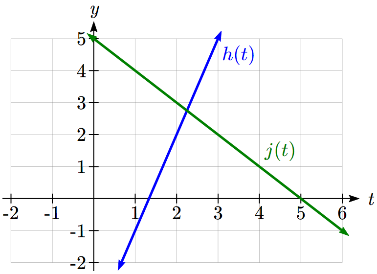
Two parallel lines can also intersect if they happen to be the same line. In that case, they intersect at every point on the lines.
3. Look at the graph in Example 7.5K above and answer the following for the function  :
:
a. Vertical intercept coordinates
b. Horizontal intercepts coordinates
c. Slope
d. Is parallel or perpendicular to (or neither)
e. Is an Increasing or Decreasing function (or neither)
f. Write a transformation description from the identity toolkit function 
Finding the intersection allows us to answer other questions as well, such as discovering when one function is larger than another.
Example 7.5L
Using the functions from the previous example, for what values of t is 
To answer this question, it is helpful first to know where the functions are equal, since that is the point where could switch from being greater to smaller than or vice-versa. From the previous example, we know the functions are equal at  .
.
By examining the graph, we can see that , the function with positive slope, is going to be larger than the other function to the right of the intersection. So when 
Give It Some Thought Answers
1.  found by starting at the vertical intercept, going up 2 units and 3 in the negative horizontal direction. You could have also answered:
  or
or  etc…
etc…
2. Parallel: 
Perpendicular: 
3. Given 
a. (0,5)
b. (5,0)
c. Slope -1
d. Neither parallel nor perpendicular
e. Decreasing function
f. Given the identity function, perform a vertical flip (over the axis) and shift up 5 units.
Section 7.5 Exercises
- Sketch the graph of the following function.

- Find the – and -intercepts of the following lines and graph the lines:
- Find the slope of the following lines and graph the lines:
- Find the equations of the lines passing through the following points, identify – and -intercepts and slope for each, and sketch their graphs.
 and
and 
 and
and 
- Consider the points
 and
and  and the linear function whose graph passes through them.
- Find the slope of the line.
- Find the slope-intercept form of the equation of the line.
- Write the equation of the line in the standard form.
- Graph
 using the vertical intercept and slope. Using the fact that the slope could also be written as , find a point on the graph that has a negative value.
 - Consider the graph of and determine the following for the function :
- Vertical intercept coordinates
- Horizontal intercepts coordinates
- Slope
- Is an increasing or decreasing function (or neither)?


7.6: Modeling with Linear Functions
When modeling scenarios with a linear function and solving problems involving quantities changing linearly, we typically follow the same problem solving strategies that we would use for any type of function:
Problem solving strategy
- Identify changing quantities, and then carefully and clearly define descriptive variables to represent those quantities. When appropriate, sketch a picture or define a coordinate system.
- Carefully read the problem to identify important information. Look for information giving values for the variables, or values for parts of the functional model, like slope and initial value.
- Carefully read the problem to identify what we are trying to find, identify, solve, or interpret.
- Identify a solution pathway from the provided information to what we are trying to find. Often this will involve checking and tracking units, building a table or even finding a formula for the function being used to model the problem.
- When needed, find a formula for the function.
- Solve or evaluate using the formula you found for the desired quantities.
- Reflect on whether your answer is reasonable for the given situation and whether it makes sense mathematically.
- Clearly convey your result using appropriate units, and answer in full sentences when appropriate.
Example 7.6A
A company purchased $120,000 in new office equipment. Then expect the value to depreciate (decrease) by $16,000 per year. Find a linear model for the value, then find and interpret the horizontal intercept and determine a reasonable domain and range for this function.
In the problem, there are two changing quantities: time and value. The remaining value of the equipment depends on how long the company has had it. We can define our variables, including units.
Output:  , value remaining, in dollars
Input: , time, in years
Reading the problem, we identify two important values. The first, $120,000, is the initial value for . The other value appears to be a rate of change – the units of dollars per year match the units of our output variable divided by our input variable. The value is depreciating, so you should recognize that the value remaining is decreasing each year and the slope is negative.
Using the intercept and slope provided in the problem, we can write the equation:

To find the horizontal intercept, we set the output to zero, and solve for the input:

The horizontal intercept is 7.5 years. Since this represents the input value where the output will be zero, interpreting this, we could say: The equipment will have no remaining value after 7.5 years.
When modeling any real life scenario with functions, there is typically a limited domain over which that model will be valid – almost no trend continues indefinitely. In this case, it certainly doesn’t make sense to talk about input values less than zero. This model is also not valid after the horizontal intercept.
The domain represents the set of input values and so the reasonable domain for this function is  . The range represents the set of output values and the value starts at $120,000 and ends with $0 after 7.5 years so the corresponding range is
  .
.
Most importantly remember that domain and range are tied together, and whatever you decide is most appropriate for the domain (the independent variable) will dictate the requirements for the range (the dependent variable).
Example 7.6B
Jamal is choosing between two moving companies. The first, U-Haul, charges an up-front fee of $20, then 59 cents a mile. The second, Budget, charges an up-front fee of $16, then 63 cents a mile[7]. When will U-Haul be the better choice for Jamal?
The two important quantities in this problem are the cost, and the number of miles that are driven. Since we have two companies to consider, we will define two functions:
Input: , miles driven
Outputs:
 : cost, in dollars, for renting from U-Haul
 : cost, in dollars, for renting from Budget
Reading the problem carefully, it appears that we were given an initial cost and a rate of change for each company. Since our outputs are measured in dollars but the costs per mile given in the problem are in cents, we will need to convert these quantities to match our desired units: $0.59 a mile for U-Haul, and $0.63 a mile for Budget.
Looking to what we’re trying to find, we want to know when U-Haul will be the better choice. Since all we have to make that decision from is the costs, we are looking for when U-Haul will cost less, or when  . The solution pathway will lead us to find the equations for the two functions, find the intersection, then look to see where the function is smaller. Using the rates of change and initial charges, we can write the equations:

These graphs are sketched to the below, with drawn dashed.
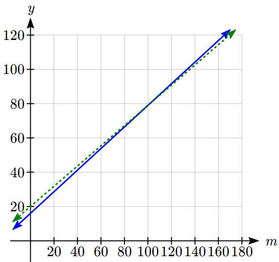
To find the intersection, we set the equations equal and solve:


This tells us that the cost from the two companies will be the same if 100 miles are driven. Either by looking at the graph, or noting that is growing at a slower rate, we can conclude that U-Haul will be the cheaper price when more than 100 miles are driven.
Example 7.6C
A company’s revenue has been growing linearly. In 2012 their revenue was $1.45 million. By 2015 the revenue had grown to $1.81 million. If this trend continues,
a. Predict the revenue in 2020
b. When will revenue reach $3 million?
The two changing quantities are the revenue and time. While we could use the actual year value as the input quantity, doing so tends to lead to very ugly equations, since the vertical intercept would correspond to the year 0, more than 2000 years ago!
To make things a little nicer, and to make our lives easier too, we will define our input as years since 2012:
Input: , years since 2012
Output:  , the company’s revenue, in millions of dollars
The problem gives us two input-output pairs. Converting them to match our defined variables, the year 2012 would correspond to  , giving the point
  . Notice that through our clever choice of variable definition, we have “given” ourselves the vertical intercept of the function. The year 2015 would correspond to , giving the point
  .
.
To predict the population in 2020 (), we would need an equation for the population. Likewise, to find when the revenue would reach $3 million, we would need to solve for the input that would provide an output of 3. Either way, we need an equation. To find it, we start by calculating the rate of change:
 million dollars per year
Since we already know the vertical intercept of the line, we can immediately write the equation:

To predict the revenue in 2020, we evaluate our function at

If the trend continues, our model predicts a revenue of $2.41 million in 2020.
To find when the population will reach $3 million, we can set  and solve for .


Our model predicts the revenue will reach $3 million in a little under 13 years after 2012, or just before the year 2025.
In business, a very common application of functions is to model cost, revenue, and profit.
Cost, Revenue, Profit
When a company produces q items, the total cost is the cost of total cost of producing those items. The total cost includes both fixed costs, which are startup costs, like equipment and buildings, and variable costs, which are costs that depend on the number of items produced, like materials and labor.
In the most simple case, Total Cost = (Fixed Costs) + (Variable Costs) ∙
Revenue is the amount of money a company brings in from sales.
In the most simple case, Revenue = (Revenue per item) ∙
Profit is the amount of money brings in, after expenses.
Profit = Revenue – Costs
We often talk about the break-even point. This is the level of production where Revenue equals Cost, or equivalently where Profit is zero. This is typically the minimum level of sales necessary for the company to make a profit.
Example 7.6D
A tech startup is looking at developing and launching a new mobile app. Initial development of the app will cost $300,000, and they estimate marketing and support for each user will cost $0.50. While the app will be free, they estimate they will be able to bring in $2 per user on average from in-app purchases. How many users will the company need to break even?
We start by modeling the cost, revenue, and profit. Let = number of users.
The fixed (initial) costs are $300,000, and the variable (per-item) costs as $0.50 per user. We can write the total cost equation:

The revenue will be $2 per user, so the revenue equation will be:

We could find the break-even point by setting the total cost equal to the revenue, which is equivalent to finding the intersection of the lines.
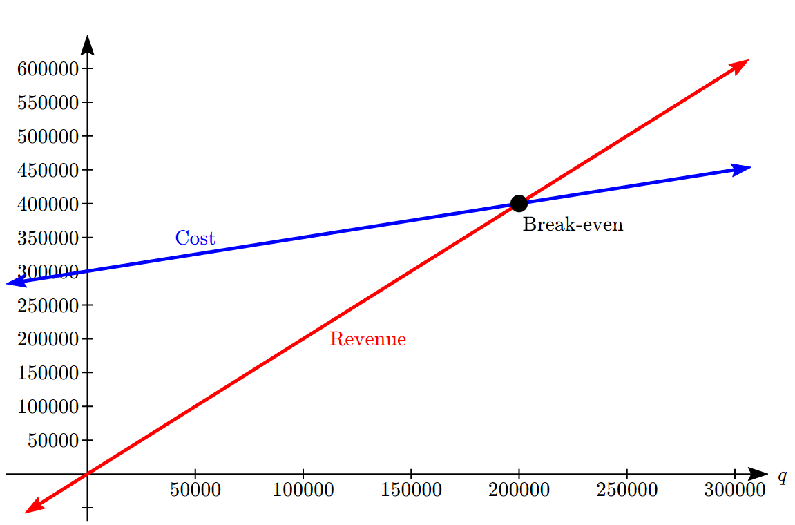
Alternatively, we could go ahead and find a profit equation first:

The break even point can be found by setting the profit equal to zero:

The company will have to acquire 200,000 users to break even.
1. A donut shop estimates their fixed daily expenses are $600. If each donut costs about $0.05 to make and sells for $0.60, how many donuts do they need to sell to break even?
In economics, there is a model for how prices are determined in a free market which states that supply and demand for a product is related to the price. The demand relationship shows the quantity of a certain product that consumers are willing to buy at a certain price. Typically the quantity demanded will decrease for an item if the price increases. The supply relationship shows the quantity of a product that suppliers are willing to produce at a certain sales price. Typically the supply demanded will increase if the price increases. Economic theory says that supply and demand will interact, and the intersection will be the equilibrium price, or market price, where the quantity supplied and demanded will be equal.
Supply and Demand
If is the price of a product, then
 is the quantity demanded
 is the quantity supplied
The demand curve is a decreasing function, while the supply curve is an increasing function.
The intersection of the curves is the equilibrium price and quantity, also called the market price and quantity. This point is often notated as  ,
,  .
.
In later chapters you will explore supply and demand curves that are non-linear, but in this chapter we will focus on linear supply and demand functions.
In most economic books, you will see the supply and demand curve written with price as the input and quantity as the output, like  . However, supply and demand graphs are drawn with price on the vertical axis and quantity on the horizontal. In an effort to avoid confusion, most of the time in this text we will instead write supply and demand curves with price as the output, to match its placement on the vertical axis.
Example 7.6E
At a price of $2.50 per gallon, there is a demand in a certain town for 42.5 thousand gallons of gas and a supply of 20 thousand gallons. At a price of $3.50, there is demand for 25.5 thousand gallons and a supply of 28 thousand gallons. Assuming supply and demand are linear, find the equilibrium price and quantity.
We start by finding a linear equation for both supply and demand. We will use price, in dollars, as the output and quantity, in thousands of gallons, as the input.
For supply, we have the points  and
and  .
.
Finding the slope:

We know the equation will look like  , so substituting in ,

The supply equation is:

For demand, we have the points  and
and  . Using a similar approach, we can find the demand equation is:

To find the equilibrium, we set the supply equal to the demand:

Multiplying through by 8(17) = 136 to clear the fractions


Now we solve for

To find the equilibrium price, we can substitute that value back into either equation:

The equilibrium quantity will be 27.2 thousand gallons of gas at a price of $3.40.
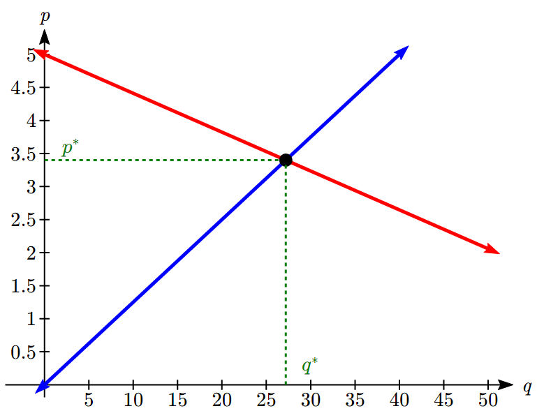
2. A company estimates that at a price of $140 there will demand for 4000 items, and for each $5 increase in price the demand will drop by 200 items. The supply curve is  . Find the equilibrium price and quantity.
Give It Some Thought Answers
1. Revenue: 
Break even when  , at a quantity of about 1091 donuts per day.
2. Demand: 
Supply = Demand when  ,
, 
Section 7.6 Exercises
- A company purchased $120,000 in new office equipment. Then expect the value to depreciate (decrease) by $16,000 per year. Find a linear model for the value of the equipment years after purchase, then find and interpret the horizontal intercept and determine a reasonable domain and range for this function.
- At a price of $2.28 per bushel, the supply of barley is 7,500 million bushels and the demand is 7,900 million bushels. At a price of $2.37 per bushel, the supply is 7,900 million bushels and the demand is 7,800 bushels.
- Assuming that price and supply are linearly related, determine the price in terms of supply (the price-supply equation).
- Assuming that price and demand are linearly related, determine the price in terms of demand (the price-demand equation).
- Find the equilibrium point (price and the number of units for which supply and demand are equal).
- Graph the price-supply equation, price-demand equation and the equilibrium point in the same coordinate system.
- Assuming that price and supply are linearly related, determine the price
- A plant can manufacture 50 tennis racquets per day for a total daily cost of $3,855 and 60 tennis racquets per day for a total daily cost of $4,245.
- Assuming that daily cost and production are linearly related, find the total daily cost of producing tennis racquets.
- Interpret the slope and the vertical intercept of this cost equation.
- Graph the total daily cost for
 .
.
- Assuming that daily cost and production are linearly related, find the total daily cost
- NewTech Wireless company offers a monthly calling plan where the total cost is linearly related to the number of minutes used. Given that the total monthly cost for 100 minutes used is
 45.00:
- Express the cost in terms of the number of minutes used .
- What are the domain and the range of this function?
- What is the basic cost for the plan and what is the cost per minute?
- Sketch the graph of this function.
- What will be the cost if 400 minutes are used in a month?
- If the total cost for a month was $40.00, how many minutes were used?
- Express the cost
- A security company purchases a new security van for $53,000 and assumes that in 5 years it will have a trade-in value of $28,000.
- Find the linear model for the depreciated value of the van after years.
- What is the depreciated value of the van after 3 years?
- When will the depreciated value fall below $23,000?
- Find the linear model for the depreciated value
- The manufacturer of a new type of frying pan has calculated the monthly fixed costs to be $83,000 and variable costs of $7.35 for each frying pan produced. The pans are sold to a distributor for $20 per pan. The monthly manufacturing capacity is 20,000 units.
- Write the monthly cost function in terms of number of units produced . Determine its domain and range and graph it.
- Write the monthly revenue function
 in terms of number of units produced . Determine its domain and range and graph it.
 - Write the monthly profit function in terms of number of units produced , assuming that all units produced are sold. Determine its domain and range and graph it.
- What will be their profit/loss if they are running at 25% capacity? At 75% capacity?
- How many units must they produce and sell in a month to break even? What percent is that of production capacity? What must be the sales to break even?
- How many units must they produce and sell in a month to make $100,000 in profit?
- Write the monthly cost function
- A manufacturing company, under contract to deliver a new line of beer bottles, estimates that it would cost $41,000 to produce 80,000 bottles while it would cost $59,000 to produce 120,000 bottles. Based on the cost analysis of previous production runs, they determined that that a linear model would best represent the costs of production.
- Assuming that the cost and the number of bottles produced are linearly related, determine the cost function
 .
. - What are the fixed costs in this model and what is the variable cost per bottle?
- Assuming that the cost
7.7: Fitting Linear Models to Data
In the real world, rarely do things follow trends perfectly. When we expect the trend to behave linearly, or when inspection suggests the trend is behaving linearly, it is often desirable to find an equation to approximate the data. Finding an equation to approximate the data helps us understand the behaviour of the data and allows us to use the linear model to make predictions about the data, inside and outside of the data range.
Example 7.7A
The table below shows the number of cricket chirps in 15 seconds, and the air temperature, in degrees Fahrenheit[8]. Plot this data, and determine whether the data appears to be linearly related.
| chirps | 44 | 35 | 20.4 | 33 | 31 | 35 | 18.5 | 37 | 26 |
| Temp | 80.5 | 70.5 | 57 | 66 | 68 | 72 | 52 | 73.5 | 53 |
Plotting this data, it appears there may be a trend, and that the trend appears roughly linear, though certainly not perfectly so.
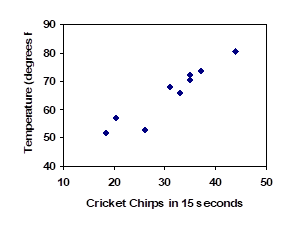
The simplest way to find an equation to approximate this data is to try to “eyeball” a line that seems to fit the data pretty well, then find an equation for that line based on the slope and intercept.
You can see from the trend in the data that the number of chirps increases as the temperature increases. As you consider a function for this data you should know that you are looking at an increasing function or a function with a positive slope.
1. a. What descriptive variables would you choose to represent Temperature & Chirps?
b. Which variable is the independent variable and which is the dependent variable?
c. Based on this data and the graph, what is a reasonable domain & range?
d. Based on the data alone, is this function one-to-one, explain?
Example 7.7B
Using the table of values from the previous example, find a linear function that fits the data by “eyeballing” a line that seems to fit.
On a graph, we could try sketching in a line. Note the scale on the axes have been adjusted to start at zero to include the vertical axis and vertical intercept in the graph.
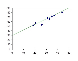
Using the starting and ending points of our “hand drawn” line, points  and
and  , this graph has a slope of
  and a vertical intercept at 30, giving an equation of

where is the number of chirps in 15 seconds, and  is the temperature in degrees Fahrenheit.
This linear equation can then be used to approximate the solution to various questions we might ask about the trend. While the data does not perfectly fall on the linear equation, the equation is our best guess as to how the relationship will behave outside of the values we have data for. There is a difference, though, between making predictions inside the domain and range of values we have data for, and outside that domain and range.
Interpolation and Extrapolation
Interpolation: When we predict a value inside the domain and range of the data
Extrapolation: When we predict a value outside the domain and range of the data
For the Temperature as a function of chirps in our hand drawn model above:
Interpolation would occur if we used our model to predict temperature when the values for chirps are between 18.5 and 44.
Extrapolation would occur if we used our model to predict temperature when the values for chirps are less than 18.5 or greater than 44.
Example 7.7C
a) Would predicting the temperature when crickets are chirping 30 times in 15 seconds be interpolation or extrapolation? Make the prediction, and discuss if it is reasonable.
b) Would predicting the number of chirps crickets will make at 40 degrees be interpolation or extrapolation? Make the prediction, and discuss if it is reasonable.
With our cricket data, our number of chirps in the data provided varied from 18.5 to 44. A prediction at 30 chirps per 15 seconds is inside the domain of our data, so would be interpolation. Using our model:
 degrees.
Based on the data we have, this value seems reasonable.
The temperature values varied from 52 to 80.5. Predicting the number of chirps at 40 degrees is extrapolation since 40 is outside the range of our data. Using our model:

Our model predicts the crickets would chirp 8.33 times in 15 seconds. While this might be possible, we have no reason to believe our model is valid outside the domain and range. In fact, generally crickets stop chirping altogether below around 50 degrees.
When our model no longer applies after some point, it is sometimes called model breakdown.
2. What temperature would you predict if you counted 20 chirps in 15 seconds?
Fitting Lines with Technology
While eyeballing a line works reasonably well, there are statistical techniques for fitting a line to data that minimize the differences between the line and data values[9]. This technique is called least-square regression, and can be computed by many graphing calculators, spreadsheet software like Excel or Google Docs, statistical software, and many web-based calculators[10].
Example 7.7D
Find the least-squares regression line using the cricket chirp data from above.
Using the cricket chirp data from earlier, with technology we obtain the equation:

Notice that this line is quite similar to the equation we “eyeballed”, but should fit the data better. Notice also that using this equation would change our prediction for the temperature when hearing 30 chirps in 15 seconds from 66 degrees to:
 degrees.
Most calculators and computer software will also provide you with the correlation coefficient, a measure of how closely the line fits the data.
Correlation Coefficient
The correlation coefficient is a value,  , between -1 and 1.
r suggests a positive (increasing) relationship
 suggests a negative (decreasing) relationship
The closer the value is to 0, the more scattered the data
The closer the value is to 1 or -1, the less scattered the data is
The correlation coefficient provides an easy way to get some idea of how close to a line the data falls.
We should only compute the correlation coefficient for data that follows a linear pattern; if the data exhibits a non-linear pattern, the correlation coefficient is meaningless. To get a sense for the relationship between the value of and the graph of the data, here are some large data sets with their correlation coefficients:
Examples of Correlation Coefficient Values
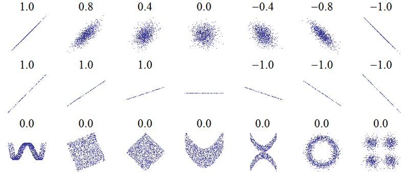
Example 7.7E
Calculate the correlation coefficient for our cricket data.
Because the data appears to follow a linear pattern, we can use technology to calculate  . Since this value is very close to 1, it suggests a strong increasing linear relationship.
Example 7.7F
Gasoline consumption in the US has been increasing steadily. Consumption data from 1994 to 2004 is shown below[12]. Determine if the trend is linear, and if so, find a model for the data. Use the model to predict the consumption in 2008.
| Year | ’94 | ’95 | ’96 | ’97 | ’98 | ’99 | ’00 | ’01 | ’02 | ’03 | ’04 |
| Consumption (billions of gallons) | 113 | 116 | 118 | 119 | 123 | 125 | 126 | 128 | 131 | 133 | 136 |
To make things simpler, a new input variable is introduced, , representing years since 1994.
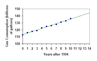
Using technology, the correlation coefficient was calculated to be 0.9965, suggesting a very strong increasing linear trend.
The least-squares regression equation is:
 .
.
Using this to predict consumption in 2008  ,
,
 billions of gallons
The model predicts 144.244 billion gallons of gasoline will be consumed in 2008.
3. Use the model created by technology in Example 7.7F to predict the gas consumption in 2011. Is this an interpolation or an extrapolation?
Give It Some Thought Answers
1. a. T = Temperature, C = Chirps (answers may vary)
b. Independent (Chirps) , Dependent (Temperature)
c. Reasonable Domain  , Reasonable Range
  (answers may vary)
d. NO, it is not one-to-one, there are two different output values for 35 chirps.
2. 54 degrees Fahrenheit
3. 150.871 billion gallons, extrapolation
Section 7.7 Exercises
Insert review exercises here
Chapter 7 Summary
Key Takeaways
Section 7.1: Functions and Function Notation
- Definition of a function
- Input (independent variable)
- Output (dependent variable)
- Function notation
- Descriptive variables
- Functions in words, tables, graphs & formulas
- Vertical line test
- Evaluating a function at a specific input value
- Solving a function given a specific output value
Section 7.2: Domain and Range
- Definition of domain
- Definition of range
- Inequalities
- Interval notation
- Set builder notation
- Domain and Range from graphs
- Piecewise defined functions
Section 7.3: Rates of Change and Behaviour of Graphs
- Rate of Change
- Average Rate of Change
- Calculating Average Rate of Change using Function Notation
- Marginal cost/revenue/profit
- Increasing/Decreasing
- Local Maxima and Minima (Extrema)
Section 7.4: Linear Functions
- Definition of a linear function
- Structure of a linear function
- Increasing & Decreasing functions
- Finding the vertical intercept
- Finding the slope/rate of change,
- Interpreting linear functions
Section 7.5: Graphs of Linear Functions
- Methods for graphing linear functions
- Another name for slope = rise/run
- Horizontal intercepts

- Horizontal lines
- Vertical lines
- Parallel lines
- Perpendicular lines
- Intersecting lines
Section 7.6: Modeling with Linear Functions
- The problem solving process
1. Identify changing quantities, and then carefully and clearly define descriptive variables to represent those quantities. When appropriate, sketch a picture or define a coordinate system.
2. Carefully read the problem to identify important information. Look for information giving values for the variables, or values for parts of the functional model, like slope and initial value.
3. Carefully read the problem to identify what we are trying to find, identify, solve, or interpret.
4. Identify a solution pathway from the provided information to what we are trying to find. Often this will involve checking and tracking units, building a table or even finding a formula for the function being used to model the problem.
5. When needed, find a formula for the function.
6. Solve or evaluate using the formula you found for the desired quantities.
7. Reflect on whether your answer is reasonable for the given situation and whether it makes sense mathematically.
8. Clearly convey your result using appropriate units, and answer in full sentences when appropriate. - Cost, revenue, profit equations
- Supply and demand
- Equilibrium price and quantity
Section 7.7: Fitting Linear Models to Data
- Fitting linear models to data by hand
- Fitting linear models to data using technology
- Interpolation
- Extrapolation
- Correlation coefficient
- http://en.wikipedia.org/wiki/Tree, retrieved July 19, 2010 ↵
- http://www.usps.com/prices/first-class-mail-prices.htm, retrieved July 19, 2010 ↵
- http://commons.wikimedia.org/wiki/File:Alaska_Crude_Oil_Production.PNG, CC-BY-SA, July 19, 2010 ↵
- https://www.pierce.ctc.edu/dist/tuition/ref/files/0910_tuition_rate.pdf, retrieved August 6, 2010 ↵
- There is also a waiting fee assessed when the taxi is waiting at red lights, but we’ll ignore that in this discussion. ↵
- http://www.thesimpledollar.com/2009/06/19/rule-1-spend-less-than-you-earn/ ↵
- Rates retrieved Aug 2, 2010 from http://www.budgettruck.com and http://www.uhaul.com/ ↵
- Selected data from http://classic.globe.gov/fsl/scientistsblog/2007/10/. Retrieved Aug 3, 2010 ↵
- Technically, the method minimizes the sum of the squared differences in the vertical direction between the line and the data values. ↵
- For example, http://www.shodor.org/unchem/math/lls/leastsq.html ↵
- http://en.wikipedia.org/wiki/File:Correlation_examples.png ↵
- http://www.bts.gov/publications/national_transportation_statistics/2005/html/table_04_10.html ↵
