8 Systems of Equations and Linear Programming
Chapter 8 Topics
8.1 Systems of Equations
8.2 Inequalities in One Variable
8.3 Linear Inequalities
8.4 Graphical Solutions
8.1: Systems of Equations
Back when studying linear equations, we found the intersection of two lines. Doing so allowed us to solve interesting problems by finding a pair of values that satisfied two different equations. While we didn’t call it this at the time, we were solving a system of equations. To start out, we’ll review an example of the type of problem we’ve solved before.
Example 8.1 A
A small business produces soap and lotion gift baskets. Labor, utilities, and other fixed expenses cost $6,000 a month. Each basket costs $8 to produce, and sells for $20. How many baskets does the company need to sell each month to break even?
In business terms, “break even” means for revenue (money brought in) to equal costs. While this problem can be approached in several ways, we’ll approach here by first creating two linear functions, one for the costs, and another for revenue.
Let’s define ![]() to be the number of gift baskets the company sells in a month. There are $6,000 of fixed costs each month, and costs increase by $8 for each basket, so we can write the linear function for costs,
to be the number of gift baskets the company sells in a month. There are $6,000 of fixed costs each month, and costs increase by $8 for each basket, so we can write the linear function for costs, ![]() , as:
, as:
![]()
Each sale brings in $20, so the revenue, ![]() , after selling
, after selling ![]() baskets will be:
baskets will be:
![]()
To find the break-even point, we are looking for the number of baskets where the revenue will equal the costs. In other words, if we were to graph the two linear functions, we are looking for the point that lies on both lines; the solution is the point that satisfies both equations.
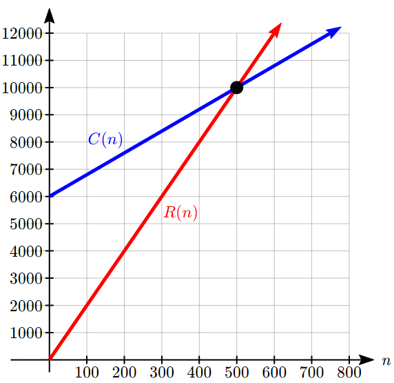
In this case we could probably solve the problem from the graph itself, but we can also solve it algebraically by setting the equations equal:
![]()
![]()
Subtract 8n from both sides:
![]()
Divide:
![]()
Evaluate either function at this input:
![]()
The break even point is at 500 baskets. The company must sell 500 baskets a month, at which point their revenue of $10,000 will cover their total costs of $10,000.
The example above illustrates one type of system of equations, one where both equations are given in functional form. When the equations are written this way, it is easy to solve the system using substitution, by setting the two outputs equal, and solving for the input. However, many system of equations problems aren’t written this way.
Example 8.1 B
A company produces a basic and premium version of its product. The basic version requires 20 minutes of assembly and 15 minutes of painting. The premium version requires 30 minutes of assembly and 30 minutes of painting. If the company has staffing for 3,900 minutes of assembly and 3,300 minutes of painting each week. If the company wants to fully utilize all staffed hours, how many of each item should they produce?
Notice first that this problem has two variables, or two unknowns – the number of basic products to make, and the number of premium products to make. There are also two constraints – the hours of assembly and the hours of painting available. This is going to give us two equations in two unknowns, what we call a 2 by 2 system of equations.
We’ll start by defining our variables:
![]() : the number of basic products produced
: the number of basic products produced
![]() : the number of premium products produced
: the number of premium products produced
Now we can create our equations based on the constraints. Each basic product requires 20 minutes of assembly, so producing ![]() items will require
items will require ![]() minutes. Each premium product requires 30 minutes of assembly, so producing
minutes. Each premium product requires 30 minutes of assembly, so producing ![]() items will require
items will require ![]() minutes. Together we have 3,900 minutes available, giving us the equation:
minutes. Together we have 3,900 minutes available, giving us the equation:
![]()
Using the same approach for painting gives the equation:
![]()
Together, these form our system of equations. They are sometimes written as a pair with a curly bracket on the left to indicate that they should be considered as connected equations.
![]()
As before, our goal is to find a pair of values, ![]() , that satisfies both equations. We’ll return to this problem and solve it shortly.
, that satisfies both equations. We’ll return to this problem and solve it shortly.
While it may not be clear, the equation ![]() we constructed above is a linear equation, like the linear equations from the first example, it’s just written differently. We could, if desired, solve this equation for
we constructed above is a linear equation, like the linear equations from the first example, it’s just written differently. We could, if desired, solve this equation for ![]() to get it written in slope-intercept form:
to get it written in slope-intercept form:
![]() ,
,
so
![]()
We typically don’t do this, since it often makes the system harder to solve then when using other techniques. To dive into this further, let’s first clarify what it means to find a solution to a system of linear equations.
System of Linear Equations
A system of linear equations consists of two or more linear equations made up of two or more variables such that all equations in the system are considered simultaneously.
A solution to a system is a set of numerical values for each variable in the system that will satisfy all equations in the system at the same time.
Not every system will have exactly one solution, but we’ll look more closely at that later. To check to see if an ordered pair is a solution to a system of equations, you would:
- Substitute the ordered pair into each equation in the system.
- Determine whether true statements result from the substitution in both equations; if so, the ordered pair is a solution.
Example 8.1 C
Determine whether the ordered pair ![]() is a solution to the given system of equations.
is a solution to the given system of equations.
![]()
Substitute the ordered pair ![]() into both equations.
into both equations.
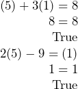
The ordered pair ![]() satisfies both equations, so it is the solution to the system.
satisfies both equations, so it is the solution to the system.
There are three common methods for solving systems of linear equations with two variables. The first is solving by graphing. In the first example above we graphed both equations, and the solution to the system was the intersection of the lines.
Example 8.1 D
Solve the following system of equations by graphing.
![]()
Solve the first equation for ![]() .
.
![]()
Solve the second equation for ![]() .
.
![]()
Graph both equations on the same set of axes.
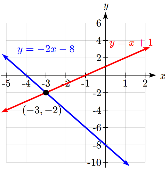
The lines appear to intersect at the point ![]() . We can check to make sure that this is the solution to the system by substituting the ordered pair into both equations.
. We can check to make sure that this is the solution to the system by substituting the ordered pair into both equations.
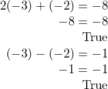
The solution to the system is the ordered pair (-3, -2).
- Solve the following system of equations by graphing.

While this method can work well enough when the solution values are both integers, it is not very useful when the intersection is not at a clear point. Additionally, it requires solving both equations for ![]() , which adds extra steps. Because of these limitations, solving by graphing is rarely used, but can be useful for checking whether your algebraic answers are reasonable.
, which adds extra steps. Because of these limitations, solving by graphing is rarely used, but can be useful for checking whether your algebraic answers are reasonable.
Solving a System by Substitution
Another method for solving a system of equations is the substitution method, in which we solve one of the equations for one variable and then substitute the result into the second equation to solve for the second variable.
Solving a system using substitution
- Solve one of the two equations for one of the variables in terms of the other.
- Substitute the expression for this variable into the second equation, then solve for the remaining variable.
- Substitute that solution into either of the original equations to find the value of the first variable. If possible, write the solution as an ordered pair.
- Check the solution in both equations.
The problem we did in Example 8.1A was technically done by substitution, but it was made easier since both equations were already solved for one variable, ![]() . An example of a more typical case is shown next.
. An example of a more typical case is shown next.
Example 8.1 E
Solve the following system of equations by substitution.
![]()
First, we will solve the first equation for ![]() .
.
![]()
Now we can substitute the expression ![]() for
for ![]() in the second equation.
in the second equation.
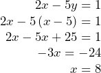
Now, we substitute ![]() into the first equation and solve for
into the first equation and solve for ![]() .
.
![]()
Our solution is ![]() .
.
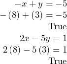
We can check the solution by substituting ![]() into both equations.
into both equations.
2. Solve the following system of equations by substitution.
![]()
Substitution can always be used, but is an especially good choice when one of the variables in one of the equations has a coefficient of 1 or -1, making it easy to solve for that variable without introducing fractions. This is fairly common in many applications.
Example 8.1 F
Julia has just retired, and has $600,000 in her retirement account that she needs to reallocate to produce income. She is looking at two investments: a very safe guaranteed annuity that will provide 3% interest, and a somewhat riskier bond fund that averages 7% interest. She would like to invest as little as possible in the riskier bond fund, but needs to produce $40,000 a year in interest to live on. How much should she invest in each account?
Notice there are two unknowns in this problem: the amount she should invest in the annuity and the amount she should invest in the bond fund. We can start by defining variables for the unknowns:
![]() : The amount (in dollars) she invests in the annuity
: The amount (in dollars) she invests in the annuity
![]() : The amount (in dollars) she invests in the bond fund.
: The amount (in dollars) she invests in the bond fund.
Our first equation comes from noting that together she is going to invest $600,000:
![]()
Our second equation will come from the interest. She earns 3% on the annuity, so the interest earned in a year would be ![]() . Likewise, the interest earned on the bond fund in a year would be
. Likewise, the interest earned on the bond fund in a year would be ![]() . Together, these need to total $40,000, giving the equation:
. Together, these need to total $40,000, giving the equation:
![]()
Together, these two equations form our system. The first equation is an ideal candidate for the first step of substitution – we can easily solve the equation for ![]() or
or ![]() :
:
![]()
Then we can substitute this expression for a in the second equation and solve.

Now substitute this back into the equation ![]() to find
to find ![]()
![]()
In order to reach her goal, Julia will have to invest $550,000 in the bond fund, and $50,000 in the annuity.
Solving a System by the Addition Method
A third method of solving systems of linear equations is the addition method, also called the elimination method. In this method, we add two terms with the same variable, but opposite coefficients, so that the sum is zero. Of course, not all systems are set up with the two terms of one variable having opposite coefficients. Often we must adjust one or both of the equations by multiplication so that one variable will be eliminated by addition.
Solving a System by the Addition Method
- Write both equations with
 – and
– and  -variables on the left side of the equal sign and constants on the right.
 - Write one equation above the other, lining up corresponding variables. If one of the variables in the top equation has the opposite coefficient of the same variable in the bottom equation, add the equations together, eliminating one variable. If not, use multiplication by a nonzero number so that one of the variables in the top equation has the opposite coefficient of the same variable in the bottom equation, then add the equations to eliminate the variable.
- Solve the resulting equation for the remaining variable.
- Substitute that value into one of the original equations and solve for the second variable.
- Check the solution by substituting the values into the other equation.
Often using the addition method will require multiplying one or both equations by a constant so terms will eliminate. Using these approaches, we can revisit the equation from Example 8.1B.
Example 8.1 G
In Example 8.1B, we set up the system below. Solve it.
![]()
Adding the equations would not eliminate a variable, but we notice that the coefficients on ![]() are the same, so multiplying one of the equations by -1 will change the sign of the coefficients. Multiplying the second equation by -1 gives the system
are the same, so multiplying one of the equations by -1 will change the sign of the coefficients. Multiplying the second equation by -1 gives the system
![]()
Adding these equations gives
![]()
Substituting ![]() = 30 into the first equation,
= 30 into the first equation,

The solution is ![]() ,
, ![]() , meaning the company should produce 120 basic products and 50 premium products to full utilize staffed hours.
, meaning the company should produce 120 basic products and 50 premium products to full utilize staffed hours.
Checking our answer in the second equation:

Give It Some Thought
3. Solve the system of equations by addition.
![]()
Example 8.1 H
Solve the given system of equations in two variables by addition.
![]()
One equation has ![]() and the other has
and the other has ![]() . The least common multiple is
. The least common multiple is ![]() so we will have to multiply both equations by a constant in order to eliminate one variable. Let’s eliminate
so we will have to multiply both equations by a constant in order to eliminate one variable. Let’s eliminate ![]() by multiplying the first equation by -5 and the second equation by 2.
by multiplying the first equation by -5 and the second equation by 2.

Then, we add the two equations together.

Substitute ![]() into the original first equation.
into the original first equation.

The solution is ![]() . Check it in the other equation.
. Check it in the other equation.

Give It Some Thought
4. Solve the system of equations by addition.
![]()
Dependent and Inconsistent Systems
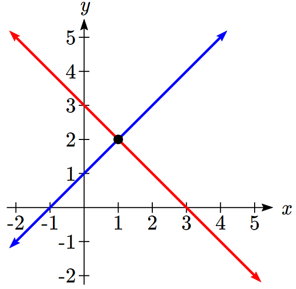
Up until now, we have only considered cases where there is exactly one solution to the system. We can categorize systems of linear equations by the number of solutions. A consistent system of equations has at least one solution. A consistent system is considered to be an independent system if it has a single solution, such as the examples we just explored. The two lines have different slopes and intersect at one point in the plane.
A consistent system is considered to be a dependent system if the equations have the same slope and the same ![]() -intercepts. In other words, the lines coincide so the equations represent the same line. Every point on the line represents a coordinate pair that satisfies the system. Thus, there are an infinite number of solutions.
-intercepts. In other words, the lines coincide so the equations represent the same line. Every point on the line represents a coordinate pair that satisfies the system. Thus, there are an infinite number of solutions.
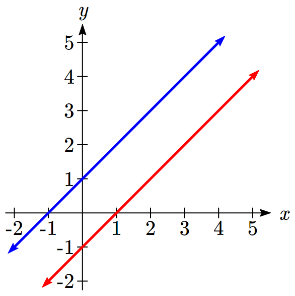
Another type of system of linear equations is an inconsistent system, which is one in which the equations represent two parallel lines. The lines have the same slope and different ![]() -intercepts. There are no points common to both lines; hence, there is no solution to the system.
-intercepts. There are no points common to both lines; hence, there is no solution to the system.
Types of Linear Systems
- An independent system has exactly one solution pair (x,y). The point where the two lines intersect is the only solution.
- An inconsistent system has no solution. Notice that the two lines are parallel and will never intersect.
- A dependent system has infinitely many solutions. The lines are coincident. They are the same line, so every coordinate pair on the line is a solution to both equations.

We can use substitution or addition to identify inconsistent systems. Recall that an inconsistent system consists of parallel lines that have the same slope but different ![]() -intercepts. They will never intersect. When searching for a solution to an inconsistent system, we will come up with a false statement, such as 12 = 0.
-intercepts. They will never intersect. When searching for a solution to an inconsistent system, we will come up with a false statement, such as 12 = 0.
Example 8.1 I
Solve the following system of equations.
![]()
We can approach this problem in two ways. Because one equation is already solved for ![]() , the most obvious step is to use substitution.
, the most obvious step is to use substitution.

Clearly, this statement is a contradiction (a false statement) because ![]() . Therefore, the system has no solution, and the system is inconsistent.
. Therefore, the system has no solution, and the system is inconsistent.
Recall that a dependent system of equations in two variables is a system in which the two equations represent the same line. Dependent systems have an infinite number of solutions because all of the points on one line are also on the other line. After using substitution or addition, the resulting equation will be an identity, such as
Example 8.1 J
Find a solution to the system of equations using the addition method.
![]()
With the addition method, we want to eliminate one of the variables by adding the equations. In this case, let’s focus on eliminating ![]() . If we multiply both sides of the first equation by -3, then we will be able to eliminate the
. If we multiply both sides of the first equation by -3, then we will be able to eliminate the ![]() -variable.
-variable.


We can see that there will be an infinite number of solutions that satisfy both equations. In some cases, realizing there are an infinite number of solutions is enough, and we can stop there. In other cases, we will want to describe the set of solutions.
One way is to simply say it’s the set of points that satisfy ![]() , but often we would solve that equation for y and describe the solution as set of points
, but often we would solve that equation for y and describe the solution as set of points ![]() .
.
Give It Some Thought
5. Solve the systems:
a.
![]()
b.
![]()
Systems with 3 variables in 3 unknowns
In systems of two variables, a solution was an ordered pair ![]() that satisfied both equations. The solution set to a three-by-three system is an ordered triple
that satisfied both equations. The solution set to a three-by-three system is an ordered triple ![]() . Graphically, the ordered triple defines the point that is the intersection of three planes in space. You can visualize such an intersection by imagining any corner in a rectangular room. A corner is defined by three planes: two adjoining walls and the floor (or ceiling). Any point where two walls and the floor meet represents the intersection of three planes.
. Graphically, the ordered triple defines the point that is the intersection of three planes in space. You can visualize such an intersection by imagining any corner in a rectangular room. A corner is defined by three planes: two adjoining walls and the floor (or ceiling). Any point where two walls and the floor meet represents the intersection of three planes.
Example 8.1K
Determine whether the ordered triple ![]() is a solution to the system.
is a solution to the system.

We will check each equation by substituting in the values of the ordered triple for ![]() ,
, ![]() , and
, and ![]() .
.
 |
 |
 |
The ordered triple ![]() is indeed a solution to the system.
is indeed a solution to the system.
We can utilize the techniques we learned in the last section to solve 3-by-3 systems of equations by reducing the problem to one we already know how to solve.
Given a linear system of three equations, solve for three unknowns
- Pick any pair of equations and solve for one variable.
- Pick another pair of equations and solve for the same variable.
- You have created a system of two equations in two unknowns. Solve the resulting two-by-two system.
- Back-substitute known variables into any one of the original equations and solve for the missing variable.
Example 8.1 L
Find a solution to the following system. The equations are numbered so we can refer to them more easily.

There will always be several choices as to where to begin, but the most obvious first step here is to eliminate ![]() by adding equations (1) and (2).
by adding equations (1) and (2).

The second step is multiplying equation (1) by ![]() and adding the result to equation (3). These two steps will eliminate the variable
and adding the result to equation (3). These two steps will eliminate the variable ![]() :
:

In equations (4) and (5), we have created a new two-by-two system. We can solve for z by adding the two equations.

Choosing one equation from each new system, we obtain the upper triangular form:

Next, we back-substitute ![]() into equation (4) and solve for
into equation (4) and solve for ![]() .
.

Finally, we can back-substitute ![]() and
and ![]() into equation (1). This will yield the solution for
into equation (1). This will yield the solution for ![]() .
.

The solution is the ordered triple ![]() .
.
Give It Some Thought
6. Solve the system of equations in three variables.

Many problems in real life depend on more than two unknowns.
Example 8.1 M
Chad is trying to plan a meal to meet specific nutritional goals. He wants to construct a dish containing rice, tofu, and peanuts that will provide 30g of protein, 14g of fat, and 50g of carbohydrates. How much of each ingredient should he use?
First off, we’re assuming any other ingredients used in the recipe aren’t contributing significantly enough to the nutrition to be considered. To answer this question, we’ll first need to know the nutritional content for the ingredients. Looking these up:
White rice: 1 cup provides: 0g fat, 44g carbohydrates, 4g protein
Tofu: 1 cup provides: 10g fat, 5g carbohydrates, 20g protein
Peanuts: 1 cup provides: 72g fat, 31g carbohydrates, 35g protein
Now we can define our variables. We are interested in the amount of each ingredient to use, so we’ll define our variables as the quantity of each ingredient:
![]() : cups of rice,
: cups of rice, ![]() : cups of tofu,
: cups of tofu, ![]() : cups of peanuts.
: cups of peanuts.
Now for each nutrient, we can create an equation. Since 1 cup of rice provides 44g carbohydrates, ![]() cups will provide
cups will provide ![]() grams of carbohydrates. Likewise
grams of carbohydrates. Likewise ![]() cups of tofu will provide
cups of tofu will provide ![]() grams, and
grams, and ![]() cups of peanuts will provide
cups of peanuts will provide ![]() grams. Together we want our recipe to provide 50g of carbohydrates, giving the equation:
grams. Together we want our recipe to provide 50g of carbohydrates, giving the equation:
![]()
Doing the same for fat and protein gives the full system:

Now we can solve the system.
Step 1. Notice that the section equation already does not involve the variable ![]() . To make things simpler, a first step might be to interchange the last two equations so the two equations with three variables will line up.
. To make things simpler, a first step might be to interchange the last two equations so the two equations with three variables will line up.

Step 2. Since ![]() is already eliminated in the last equation, we’ll eliminate
is already eliminated in the last equation, we’ll eliminate ![]() from the first two equations. Multiply equation (2) by -11.
from the first two equations. Multiply equation (2) by -11.

Step 3. Add equations (1) and (2), writing the result as row 2.

Step 4. Multiply equation (2) by 2 and equation (3) by 43.

Step 5. Add equations (2) and (3), writing the result in row 3.

Step 6. Solve for ![]() in equation 3. For a real life problem like this, decimal approximations are probably fine.
in equation 3. For a real life problem like this, decimal approximations are probably fine.
![]()
Step 7. Back substitute the value for ![]() into equation (2) to solve for
into equation (2) to solve for ![]() .
.

Step 8. Back substitute the values for ![]() and
and ![]() into equation (1) and solve for
into equation (1) and solve for ![]() .
.

To meet his nutritional goals, Chad should use 0.979 cups of rice, 1.273 cups of tofu, and 0.0176 cups of peanuts.
This particular system was rather unpleasant to solve. In the rest of the chapter we will learn some other techniques for solving complex systems.
Give It Some Thought Answers
1. The solution to the system is the ordered pair ![]() .
.
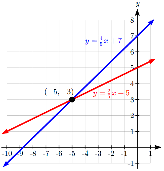
2. ![]()
3. ![]()
4. ![]()
5. a. No solution. The system is inconsistent.
b. The system is dependent so there are infinite solutions of the form ![]() .
.
6. ![]()
Section 8.1 Exercises
- Solve each of the following systems of equations.
- Kayla and Amina agree to form a partnership which requires Amina to invest $6,465 less than three-quarters of what Kayla is to invest. If the total partnership value is $61,243, how much did each partner invest?
- A college theatre collected $1,300 from the sale of 450 tickets. If the tickets were sold for
 3.50, how many tickets were sold at each price?
 - An employee gets paid $16 per hour. Last week, the employee’s weekly total of regular hours and overtime hours at time-and-a-half were 44 and the total compensation was $800. How many regular and overtime hours did the employee work?
- A furniture company has been producing 93 bedside tables day working two shifts. The second shift has produced 33 bedside tables fewer than five-halves of the number of bedside tables produced by the first shift. Determine the number of bedside tables each shift has produced.
- Eyad diversified his investment so that part of his investment earns interest at rate of 4% per annum, and part earns 6% per annum. If the total annual interest on the investment is $560, and he invests twice as much at 4% as he invests at 6%, how much did Eyad invest at each rate?
- The Kirkland Company markets two products. Each unit of Product A requires five units of labour, while each unit of Product B requires two units of labour. Two hundred units of labour are available per time period. How many of each product can they market?
- Nancy’s sales last week were $140 less than three times Andrea’s sales. Together they sold $940. How much did each sell last week?
- A political candidate has budgeted $10,000 to spend on radio and television advertising. A radio ad costs $200 per 30-second spot, and a television ad costs $800 per 30-second spot. How many radio and television spots can the candidate purchase for $10,000 if they want to run as many radio spots as television spots?
- A restaurant offered two dinner specials. The difference between seven times the orders for the first dinner special and four times the orders for the second special is 12. The sum of the three-fourths of the orders for the first special and two-thirds of the orders for the second special is 21. Find the number of orders for each special.
- A manufacturing plant makes two types of inflatable boats – a two-person boat and a four-person boat. Each two-person boat requires 0.9 labour-hours in the cutting department and 0.8 labour hours in the assembly department. Each four-person boat requires 1.8 labour-hours in the cutting department and 1.2 labour hours in the assembly department. The monthly total number of labour-hours in the cutting and the assembly departments are 864 and 672 respectively. How many of each type of boat can the plant manufacture?
- A human resource manager is trying to estimate the cost of a workforce accident. These costs usually consist of direct costs (such as medical bills, equipment damage, and legal expenses) and indirect costs (such as decreased output, production delays, and fines). From past experience, she knows that indirect costs average six times as much as direct costs. If she estimates the cost of an accident to be $21,000, what is the direct cost of the accident?
- St. Boniface Hospital raises funds for research through its Mega Lottery program. In this program, 16,000 tickets are available for purchase at a price of one for $100 or three for $250. This year, the lottery sold out with sales of $1,506,050. To better plan next year’s lottery, the marketing manager wants to know how many tickets were purchased under each option this year.
- An accountant is trying to allocate production costs from two different products to their appropriate ledgers. Unfortunately, the production log sheet for last week has gone missing. However, from other documents he was able to figure out that 1,250 units in total were produced last week. The production machinery was run for 2,562.5 minutes, and he knows that Product A takes 1.5 minutes to manufacture while Product B takes 2.75 minutes to manufacture. How many units of each product were produced last week?
- A 240 mL bottle of an orange drink claims that it is made with real fruit juice. Upon examination of the ingredient list, only 15% of the contents is actually fruit juice. How many milliliters of “other ingredients” are in the bottle?
- Goodyear Tires just completed a “Buy Three Get One Free” promotion on its ultra-grip SUV tires, regularly priced at $249.99 per tire. Over the course of the promotion, 1,405 tires were sold resulting in sales of $276,238.95. How many tires were sold at the regular price and how many tires were sold at the special promotional price?
- A local baseball team sells tickets with two price zones. Seats behind the plate from first base to third base are priced at $20 per ticket. All other seats down the base lines and in the outfield are priced at $10 per ticket. At last night’s game, 5,332 fans were in attendance and total ticket revenue was $71,750. How many tickets in each zone were sold?
- Marianne, William, Hendrick, and Charlotte have all decided to go into business together. They need $175,000 in initial capital funding. William was able to contribute 20% less than Marianne, Hendrick contributed 62.5% more than William, and Charlotte contributed $5,000 less than half as much as Marianne. How much did each partner contribute to the initial funds?
- A mall is being constructed and needs to meet the legal requirements for parking availability. Parking laws require one parking stall for every 100 square feet of retail space. The mall is designed to have 1,200,000 square feet of retail space. Of the total parking stalls available, 2% need to be handicap accessible, there need to be three times as many small car spaces as handicap spaces, RV spaces need to be one-quarter of the number of small car spaces, and the rest of the spaces are for regular stalls. How many of each type of parking space does the mall require?
8.2: Inequalities in One Variable
When learning about domain and range, you learned about inequalities and using set-builder and interval notation to represent them. In this section, we will explore how to solve linear and absolute value inequalities in one variable. The process is very similar to solve equations, but instead of the solution being a single value, the solution will be an inequality.
Notice that if an inequality is true, like 2 < 5, then these operations result in a true statement as well, just like with equations:
Adding a number to both sides:

Subtracting a number on both sides:

Multiplying a positive number on both sides:

Dividing by a positive number on both sides:

We can use these operations just like when solving equations.
Example 8.2A
Solve ![]()
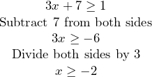
This inequality represents the solution set. It tells us that all numbers greater than or equal to -2 will satisfy the original inequality. We could also write this solution in interval notation, as ![]()
To understand what is happening, we could also consider the problem graphically. If we were to graph the equation ![]() , then solving
, then solving ![]() would correspond with asking “for what values of
would correspond with asking “for what values of ![]() is
is ![]() ”.
”.
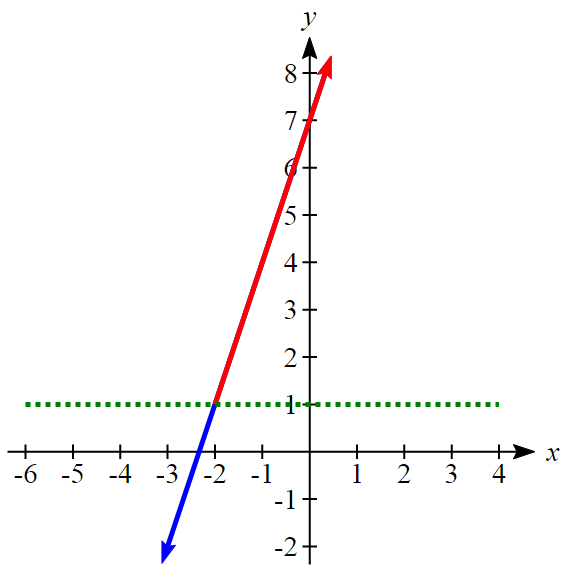
Notice that the part of the graph where this is true corresponds to where ![]() .
.
While most operations in solving inequalities are the same as in solving equations, we run into a problem when multiplying or dividing both sides by a negative number. Notice, for example:

To account for this, when multiplying or dividing by a negative number, we must reverse the sign of the inequality.
Rules for Solving Linear Inequalities
- You may add or subtract a positive or negative number to both sides of the inequality.
- You can multiply or divide both sides of the inequality by a positive number.
- You can multiply or divide both sides of the inequality by a negative number, but you must reverse the direction of the inequality.
Example 8.2B
Solve ![]()

Give It Some Thought
1. Solve: ![]()
Example 8.2C
A company spends $1200 per day on overhead and labor, and each item they produce costs $5 for materials. If they sell the items for $15 each, how many items will they need to sell each day for their profits to be positive?
While we could solve this problem using equations, it also lends itself to inequalities, since we want the profit to be positive: ![]() .
.
Costs: ![]()
Revenue: ![]()
Profit: ![]()
Solving ![]() :
:

The company will need to less at least 240 items a day to make a profit.
Compound Inequalities
Compound inequalities are inequalities that consist of more than one part. The most common type is called a tripartite inequality. The basic version looks like this: ![]() .
.
When we write these it is important that both inequalities point in the same direction and that the “outside” inequality is also true – in this case ![]() is true, so this is valid. Expressions like
is true, so this is valid. Expressions like ![]() and
and ![]() are not valid notation.
are not valid notation.
The most universal way to solve a tripartite inequality is to:
- Break it into two separate inequalities
- Solve each inequality separately
- Combine the solutions if possible.
Example 8.2D
Solve ![]()
First we separate this into two inequalities:
![]()
and
![]()
Now we solve each:
![]()
and
![]()
Now we can combine these solution sets. The numbers where both ![]() and
and ![]() are true is the set:
are true is the set:
![]()
While this solution is valid and correct, it is more common to write the solution to tripartite inequalities with the smaller number on the left. We could rewrite the solution as:
![]()
This also has the advantage of corresponding better with the answer in interval notation: ![]() .
.
With this particular inequality, it would also be possible to skip the step of breaking it apart, and instead just subtract 5 from all three “parts” of the inequality. This works for simple problems like this, but may fail if the inequality has variables in more than one “part” of the inequality.
Give It Some Thought
2. Solve: ![]()
Absolute Value
So far in this section we have been looking at inequalities that are linear. We will now turn to absolute value inequalities. The absolute value function is a piecewise-defined function made up of two linear functions.
Absolute Value Function
The absolute value function can be defined as
![]()
The graph of the absolute value looks like a V:
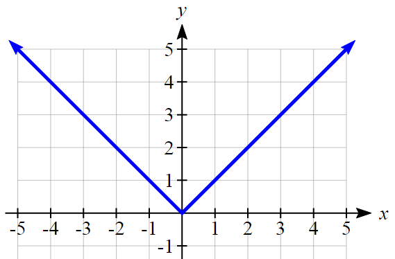
The absolute value function is commonly used to determine the distance between two numbers on the number line. Given two values ![]() and
and ![]() , then
, then ![]() will give the distance, a positive quantity, between these values, regardless of which value is larger.
will give the distance, a positive quantity, between these values, regardless of which value is larger.
Example 8.2E
Describe all values, ![]() , within a distance of 4 from the number 5.
, within a distance of 4 from the number 5.
We want the distance between ![]() and 5 to be less than or equal to 4. The distance can be represented using the absolute value, giving the expression
and 5 to be less than or equal to 4. The distance can be represented using the absolute value, giving the expression
![]()
Example 8.2 F
A 2010 poll reported 78% of Americans believe that people who are gay should be able to serve in the US military, with a reported margin of error of 3%[1]. The margin of error tells us how far off the actual value could be from the survey value[2]. Express the set of possible values using absolute values.
Since we want the size of the difference between the actual percentage, ![]() , and the reported percentage to be less than 3%,
, and the reported percentage to be less than 3%,
![]()
Give It Some Thought
3. Students who score within 20 points of 80 will pass the test. Write this as a distance from 80 using the absolute value notation.
Solving Absolute Value Equations
To solve an equation like ![]() , we can notice that the absolute value will be equal to 8 if the quantity inside the absolute value were 8 or -8. This leads to two different equations we can solve independently:
, we can notice that the absolute value will be equal to 8 if the quantity inside the absolute value were 8 or -8. This leads to two different equations we can solve independently:

or

Solutions to Absolute Value Equations
An equation of the form ![]() , with
, with ![]() , will have solutions when
, will have solutions when ![]() or
or ![]() .
.
Example 8.2G
Solve: ![]()


or

There are two solutions: ![]() and
and ![]()
Example 8.2H
Solve ![]()
Isolating the absolute value on one side the equation,

At this point, we notice that this equation has no solutions – the absolute value always returns a positive value, so it is impossible for the absolute value to equal a negative value.
Give It Some Thought
4. Find the horizontal & vertical intercepts for the function
![]()
Solving Absolute Value Inequalities
When absolute value inequalities are written to describe a set of values, like the inequality ![]() we wrote earlier, it is sometimes desirable to express this set of values without the absolute value, either using inequalities, or using interval notation.
we wrote earlier, it is sometimes desirable to express this set of values without the absolute value, either using inequalities, or using interval notation.
We will explore two approaches to solving absolute value inequalities:
- Using a graph
- Using test values
Example 8.2I
Solve ![]()
With both approaches, we will need to know first where the corresponding equality is true. In this case we first will find where ![]() . We do this because the absolute value is a nice friendly function with no breaks, so the only way the function values can switch from being less than 4 to being greater than 4 is by passing through where the values equal 4. Solve
. We do this because the absolute value is a nice friendly function with no breaks, so the only way the function values can switch from being less than 4 to being greater than 4 is by passing through where the values equal 4. Solve ![]() ,
,
![]()
or
![]()
To use a graph, we can sketch the function ![]() . To help us see where the outputs are 4, the line
. To help us see where the outputs are 4, the line ![]() could also be sketched.
could also be sketched.
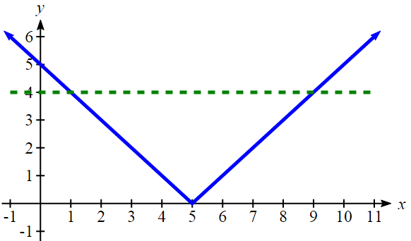
On the graph, we can see that indeed the output values of the absolute value are equal to 4 at ![]() and
and ![]() . Based on the shape of the graph, we can determine the absolute value is less than or equal to 4 between these two points, when
. Based on the shape of the graph, we can determine the absolute value is less than or equal to 4 between these two points, when ![]() . In interval notation, this would be the interval
. In interval notation, this would be the interval ![]() .
.
As an alternative to graphing, after determining that the absolute value is equal to 4 at ![]() and
and ![]() , we know the graph can only change from being less than 4 to greater than 4 at these values. This divides the number line up into three intervals:
, we know the graph can only change from being less than 4 to greater than 4 at these values. This divides the number line up into three intervals: ![]() ,
, ![]() , and
, and ![]() . To determine when the function is less than 4, we could pick a value in each interval and see if the output is less than or greater than 4.
. To determine when the function is less than 4, we could pick a value in each interval and see if the output is less than or greater than 4.
| Interval | Test |
<4 or >4? | |
| 0 | greater | ||
| 6 | less | ||
| 11 | greater |
Since ![]() is the only interval in which the output at the test value is less than 4, we can conclude the solution to
is the only interval in which the output at the test value is less than 4, we can conclude the solution to ![]() is
is ![]() .
.
Example 8.2J
Given the function ![]() , determine for what
, determine for what ![]() values the function values are negative.
values the function values are negative.
We are trying to determine where ![]() , which is when
, which is when ![]() . We begin by isolating the absolute value:
. We begin by isolating the absolute value:

Next we solve for the equality ![]()

or

We can now either pick test values or sketch a graph of the function to determine on which intervals the original function value are negative. Notice that it is not even really important exactly what the graph looks like, as long as we know that it crosses the horizontal axis at ![]() and
and ![]() , and that the graph has been flipped.
, and that the graph has been flipped.
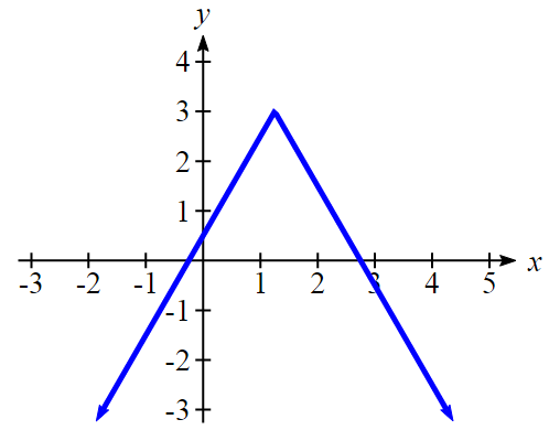
From the graph of the function, we can see the function values are negative to the left of the first horizontal intercept at ![]() , and negative to the right of the second intercept at
, and negative to the right of the second intercept at ![]() . This gives us the solution to the inequality:
. This gives us the solution to the inequality:
![]()
In interval notation, this would be ![]()
Give It Some Thought
6. Solve ![]()
There is a third approach to solving absolute value inequalities that is formulaic. While it works, and you are welcome to use it, it is much more likely that you will remember the other approaches.
Solutions to Absolute Value Inequalities
To solve ![]() , solve:
, solve: ![]()
To solve ![]() , solve:
, solve: ![]() or
or ![]()
Example 8.2K
Solve ![]()
We need to start by isolating the absolute value:
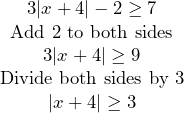
Now we can break this apart and solve each piece separately:
![]()
or
![]()
In interval notation, this would be ![]()
Give It Some Thought Answers
1. ![]()
2. ![]()
3. Using the variable ![]() , for passing,
, for passing, ![]()
4. ![]()
5. ![]() , so the vertical intercept is at
, so the vertical intercept is at ![]() .
.
![]() when
when ![]() and
and ![]() so the horizontal intercepts are at
so the horizontal intercepts are at ![]() and
and ![]() .
.
6. ![]() or
or ![]() ; in interval notation this would be
; in interval notation this would be ![]()
Section 8.2 Exercises
- Solve each inequality and write the solution set using interval form and graph it.
- Use graph solution notation to write the following using single interval, if possible.
- Solve the following inequalities and describe the solutions using set, interval and graph notation:
- Solve each compound inequality. Write the solution set using interval notation and graph it.
 and
and 
 and
and 
 and
and 
 or
or 
 or
or 
 or
or 
 and
and 
 and
and 


- Write an inequality to describe the following situation: Kate will buy the jacket provided the cost
 is at most $117.
 - A company spends $1200 per day on overhead and labor, and each item they produce costs $5 for materials. If they sell the items for $15 each, how many items will they need to sell each day for their profits to be positive?
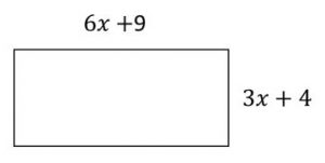
- Consider the following rectangle. For what values of (measured in cm) will the rectangle have the perimeter of at least 242 cm?
- For what values of
 is each of the following expressions a real number?
- A student scored 67 points on his Psychology 101 midterm. If the average of his midterm and final must be between 79 and 90 inclusive for a B, then for what range of scores on the final exam would a student get a B? Both tests have a maximum of 100 points. Write your answer in interval
- To receive a B in a math course, an average between 80 and 89, inclusive, is required. Leah has scores of 76, 82 and 90 on her first three math tests. After the fourth test, she states that she now has a B average. In what range was her score on the fourth test for this statement to be true? Write your answer in interval notation.
- To mail an envelope, Canada Post charges 37 cents for the first gram, and 25 cents for each additional gram. What is the weight of the envelope that can be mailed for $8.35? Write your answer in interval notation.
- A car rents for $45 per day plus 21 ¢ per kilometer. You are at a daily budget of $66. How many kilometers can you cover to stay within your budget?
- Anna is considering writing and publishing her own book. She estimates her revenue to be
 and her cost to be
  where
where  is the number of books sold. Find the minimum number of books she must sell to make a profit.
 - Jan scored 65 points on the calculus midterm. If the final exam counts twice as much as the midterm exam, then what range of the final exam scores would result in the final average between 79 and 90? Both tests have a maximum of 100 points. Write your answer in interval form.
- Canada post defines girth of a box as the sum of the twice the width and twice the width. The maximum length, height and width allowed are 2 m and length plus girth must be at most 3 m. If the box is 1 m long and 75 cm wide, in what range can the height be?
8.3: Linear Inequalities
In the systems of equations section, we looked at a company that produces a basic and premium version of its product, and we determined how many of each item they should produce to fully utilize all staffed hours. In some cases, though, it might not make the most sense for the company to utilize all the staffed hours; if the premium product has high demand and a high price, it might make more sense for the company to make as many of those, even if some staff hours go unused. In this case, the company might be most interested in what combinations of basic and premium product production are possible. For that, we need linear inequalities.
A linear equation in two variables is an equation like ![]() , which is sometimes written without function notation as
, which is sometimes written without function notation as ![]() . Recall that the graph of this equation is a line, formed by all the points
. Recall that the graph of this equation is a line, formed by all the points ![]() that satisfy the equation. A linear inequality in two variables is similar, but involves an inequality. Some examples:
that satisfy the equation. A linear inequality in two variables is similar, but involves an inequality. Some examples:
![]()
![]()
![]()
![]()
Linear inequalities can also be written with both variables on the same side of the equation, like ![]() .
.
The solution set to a linear inequality will be all the points ![]() that satisfy the inequality. Notice that the line
that satisfy the inequality. Notice that the line ![]() divides the coordinate plane into two halves; on one half
divides the coordinate plane into two halves; on one half ![]() , and on the other
, and on the other ![]() . The solution set to a linear inequality will be a half plane, and to show the solution set we shade the part of the coordinate plane where the points lie in the solution set.
. The solution set to a linear inequality will be a half plane, and to show the solution set we shade the part of the coordinate plane where the points lie in the solution set.
To graph the solution to a linear inequality
- If necessary, rewrite the linear inequality into a form convenient for graphing, like slope-intercept form.
- Graph the corresponding linear equation.
a. For a strict inequality (< or >), draw a dashed line to show that the points on the line are not part of the solution
b. For an inequality that includes the equal sign (≤ or ≥), draw a solid line to show that the points on the line are part of the solution. - Choose a test point, not on the line.
a. Substitute the test point into the inequality
b. If the inequality is true at the test point, shade the half plane on the side including the test point
c. If the inequality is not true at the test point, shade the half plane on the side that doesn’t include the test point.
Example 8.3A
Graph the solution to ![]()
Since this is a strict inequality, we will graph ![]() as a dashed line.
as a dashed line.
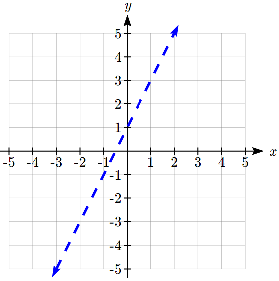
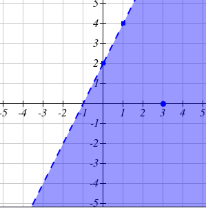
Now we choose a test point not on the line. Usually picking a point where one coordinate is zero will make things easier. Let’s use ![]() .
.
Substituting ![]() into the inequality, we get
into the inequality, we get
![]()
This is a true statement, so we will shade the side of plane that includes ![]()
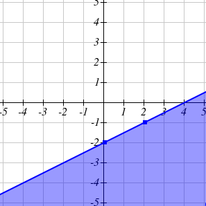
Example 8.3B
Graph the solution to ![]()
This is not written in a form we are used to use for graphing, so we might solve it for ![]() first.
first.
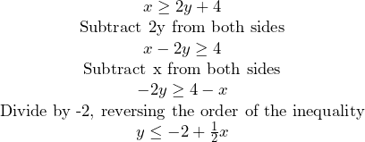
Since this inequality includes the equals sign, we will graph ![]() as a solid line.
as a solid line.
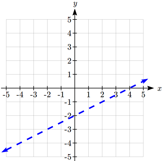
Now we choose a test point not on the line. ![]() is a convenient choice. Substituting
is a convenient choice. Substituting ![]() into the inequality, we get
into the inequality, we get
![]()
This is a false statement, so we shade the half of the plane that does not include ![]() .
.
Give It Some Thought
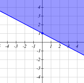
1. Graph the solution to ![]()
Example 8.3C
A store sells peanuts for $4/pound and cashews for $8/pound, and plans to sell a new mixed-nut blend in a jar. What combinations of peanuts and cashews are possible, if they want the mix to cost $6 or less?
We start by defining our variables:
![]() : The number of pounds of peanuts in 1 pound of mix
: The number of pounds of peanuts in 1 pound of mix
![]() : The number of pounds of cashews in 1 pound of mix
: The number of pounds of cashews in 1 pound of mix
The cost of one pound of mix will be ![]() , so all the mixes costing $6 or less will satisfy the inequality
, so all the mixes costing $6 or less will satisfy the inequality ![]() .
.
We can graph the equation ![]() fairly easily by finding the intercepts:
fairly easily by finding the intercepts:
When ![]() = 0,
= 0,

So the point ![]() is on the line.
is on the line.
When ![]() ,
, ![]() , so
, so ![]() , giving the point
, giving the point ![]() .
.
Notice the test point ![]() will satisfy the inequality, so we will shade the side of the line including the origin.
will satisfy the inequality, so we will shade the side of the line including the origin.
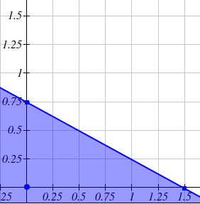
Because of the context, only values in the first quadrant are reasonable. The graph shows all the possible combinations the store could use, including 1 pound of peanuts with 1/4 pound of cashews, or 1/2 a pound of each.
Systems of Linear Inequalities
In the systems of equations chapter, we looked for solutions to a system of linear equations – a point that would satisfy all the equations in the system. Likewise, we can consider a system of linear inequalities. The solution to a system of linear inequalities is the set of points that satisfy all the inequalities in the system.
With a single linear inequality, we can show the solution set graphically. Likewise, with a system of linear inequalities we show the solution set graphically. We find it by looking for where the regions indicated by the individual linear inequalities overlap.
Example 8.3D
Graph the solution to the system of linear inequalities
![]()
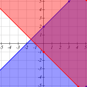
If we graph the solution set to each inequality individually, we get the two solutions sets shown here.
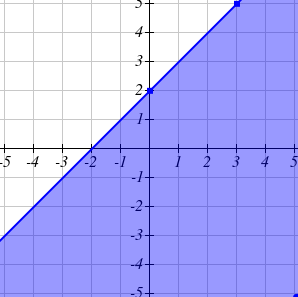
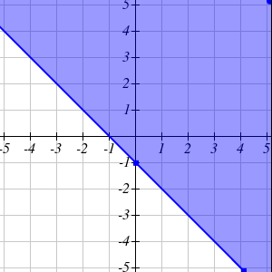
Graphing these solution sets on the same axes reveals the solution to the system of inequalities as the region where the two overlap.
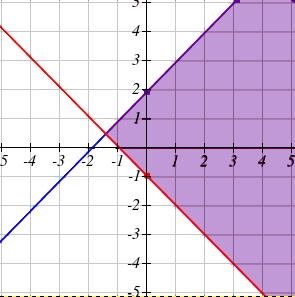
The solution set, where the regions overlap:
The solution set, drawn alone:
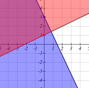
2. Graph the solution to the system of linear inequalities
![]()
The following question is similar to a problem we solved using systems in the systems chapter.
Example 8.3E
A company produces a basic and premium version of its product. The basic version requires 20 minutes of assembly and 15 minutes of painting. The premium version requires 30 minutes of assembly and 30 minutes of painting. If the company has staffing for 3,900 minutes of assembly and 3,300 minutes of painting each week. How many items can then produce within the limits of their staffing?
Notice this problem is different than the question we asked in the first section, since we are no longer concerned about fully utilizing staffing, we are only interested in what is possible. As before, we’ll define
![]() : The number of basic products made
: The number of basic products made
![]() : The number of premium products made.
: The number of premium products made.
Just as we created equations in the first section, we can now create inequalities, since we know the hours used in production needs to be less than or equal to the hours available. This leads to two inequalities:
![]()
Graphing these inequalities gives us the solution set.
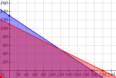
Since it isn’t reasonable to consider negative numbers of items, we can further restrict the solutions to the first quadrant. This could also be represented by adding the inequalities ![]() and
and ![]() .
.
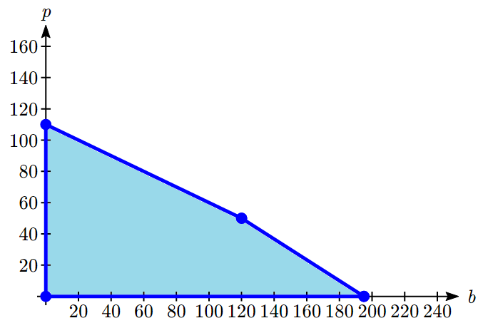
In the solution set we can see the solution to the system of equations we solved in the previous section: 120 basic products and 50 premium products. The solution set shows that if the company is willing to not fully utilize the staffing, there are many other possible combinations of products they could produce.
The techniques we used above are key to a branch of mathematics called linear programming, which is used extensively in business. We will explore linear programming further in the next section.
Give It Some Thought Answers
1. 
2. 
Section 8.3 Exercises
- Graph by hand the solution region of each of the following systems of inequalities, identify its corner points and state whether the region is bounded or unbounded.
8.4: Graphical Solutions
Wouldn’t it be nice if we could simply produce and sell infinitely many units of a product and thus make a never-ending amount of money? In business (and in day-to-day living) we know that some things are just unreasonable or impossible. Instead, our hope is to maximize or minimize some quantity, given a set of constraints.
In order to have a linear programming problem, we must have:
- Constraints, represented as inequalities
- An objective function, that is, a function whose value we either want to be as large as possible (want to maximize it) or as small as possible (want to minimize it).
Consider this extension of the example from the end of the last section.
Example 8.4A
A company produces a basic and premium version of its product. The basic version requires 20 minutes of assembly and 15 minutes of painting. The premium version requires 30 minutes of assembly and 30 minutes of painting. If the company has staffing for 3,900 minutes of assembly and 3,300 minutes of painting each week. They sell the basic products for a profit of $30 and the premium products for a profit of $40. How many of each version should be produced to maximize profit?
Let ![]() = the number of basic products made, and
= the number of basic products made, and ![]() = the number of premium products made. Our objective function is what we’re trying to maximize or minimize. In this case, we’re trying to maximize profit. The total profit,
= the number of premium products made. Our objective function is what we’re trying to maximize or minimize. In this case, we’re trying to maximize profit. The total profit, ![]() , is
, is
![]()
In the last section, the example developed our constraints. Together, these define our linear programming problem:
Objective function: ![]()
Constraints:

In this section, we will approach this type of problem graphically. We start by graphing the constraints to determine the feasible region – the set of possible solutions. Just showing the solution set where the four inequalities overlap, we see a clear region.
To consider how the objective function connects, suppose we considered all the possible production combinations that gave a profit of ![]() = $3000, so that
= $3000, so that ![]() . That set of combinations would form a line in the graph. Doing the same for a profit of $5000 and $6500 would give additional lines. Graphing those on top of our feasible region, we see a pattern:
. That set of combinations would form a line in the graph. Doing the same for a profit of $5000 and $6500 would give additional lines. Graphing those on top of our feasible region, we see a pattern:
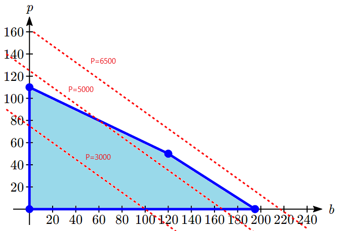
Notice that all the constant-profit lines are parallel, and that in general the profit increases as we move up to upper right. Notice also that for a profit of $5000 there are some production levels inside the feasible region for that profit level, but some are outside. That means we could feasibly make $5000 profit by producing, for example, 167 basic items and no premium items, but we can’t make $5000 by producing 125 premium items and no basic items because that falls outside our constraints.
The solution to our linear programming problem will be the largest possible profit that is still feasible. Graphically, that means the line furthest to the upper-right that still touches the feasible region on at least point. That solution is the one below:
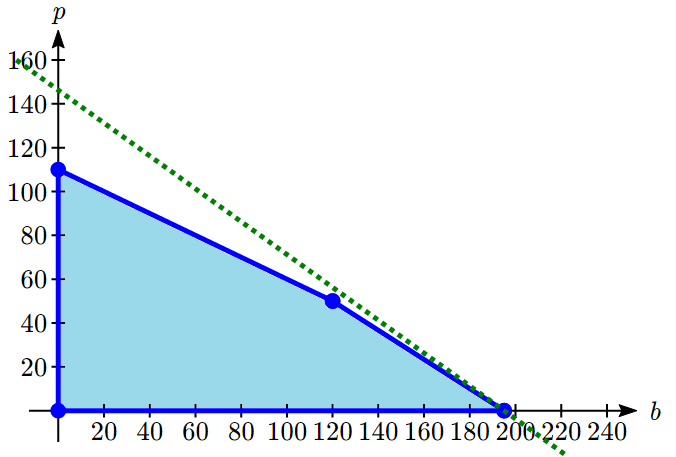
This profit line touches the feasible region where ![]() and
and ![]() , giving a profit of
, giving a profit of ![]() = 30(195) + 40(0) = $5850.
= 30(195) + 40(0) = $5850.
Notice that this is slightly larger than the profit that would be made by completely utilizing all staffing at ![]() ,
, ![]() , where the profit would be $5600.
, where the profit would be $5600.
The objective function along with the four corner points above forms a bounded linear programming problem. That is, imagine you are looking at three fence posts connected by fencing (black point and lines, respectively). If you were to put your dog in the middle, you could be sure it would not escape (assuming the fence is tall enough). If this is the case, then you have a bounded linear programming problem. If the dog could walk infinitely in any one direction, then the problem is unbounded.
In the past example, you can see that the line of maximum profit will always touch the boundary of the feasible region. That observation inspires the fundamental theorem of linear programming.
Fundamental Theorem of Linear Programming
- If a solution exists to a bounded linear programming problem, then it occurs at one of the corner points.
- If a feasible region is unbounded, then a maximum value for the objective function does not exist.
- If a feasible region is unbounded, and the objective function has only positive coefficients, then a minimum value exists.
In the last example we solve the problem somewhat intuitively by “sliding” the profit line up. Typically we use a more procedural approach.
Solving a Linear Programming Problem Graphically
- Define the variables to be optimized. The question asked is a good indicator as to what these will be.
- Write the objective function, first in words, then convert to a mathematical equation
- Write the constraints, first in words, then convert to mathematical inequalities
- Graph the constraints inequalities, and shade the feasible region
- Identify the corner points by solving systems of linear equations whose intersection represents a corner point.
- Test all corner points in the objective function. The “winning” point is the point that optimizes the objective function (biggest if maximizing, smallest if minimizing)
Give It Some Thought
1. Maximize ![]() subject to the constraints:
subject to the constraints:

Example 8.4B
A health-food business would like to create a high-potassium blend of dried fruit in the form of a box of 10 fruit bars. It decides to use dried apricots, which have 407 mg of potassium per serving, and dried dates, which have 271 mg of potassium per serving. The company can purchase its fruit in bulk for a reasonable price. Dried apricots cost $9.99/lb. (about 3 servings) and dried dates cost $7.99/lb. (about 4 servings). The company would like the box of bars to have at least the recommended daily potassium intake of about 4700 mg, and contain at least 1 serving of each fruit. In order to minimize cost, how many servings of each dried fruit should go into the box of bars?
We begin by defining the variables. Let
![]() = number of servings of dried apricots
= number of servings of dried apricots
![]() = number of servings of dried dates
= number of servings of dried dates
We next work on the objective function.
For apricots, there are 3 servings in one pound. This means that the cost per serving is $9.99/3 = $3.33. The cost for ![]() servings would thus be
servings would thus be ![]() .
.
For dates, there are 4 servings per pound. This means that the cost per serving is $7.99/4 = $2.00. The cost for ![]() servings would thus be
servings would thus be ![]() .
.
The total cost, ![]() , for apricots and dates would be
, for apricots and dates would be ![]()
Normally we would have constraints ![]() and
and ![]() since negative servings can’t be used. But in this case, we’re further restricted. In words:
since negative servings can’t be used. But in this case, we’re further restricted. In words:
- There must be at least 1 serving of each fruit
- The product must contain at least 4700 mg of potassium
Mathematically,
- Since there must be at least 1 serving of each fruit,
 and
and 
- There are
 mg of potassium in
  servings of apricots and
  mg of potassium in
  servings of dates. The sum should be greater than or equal to 4700 mg of potassium, or
Thus we have,
Objective function:
![]()
Constraints:
![]()
We graph the constraints and shade the feasible region:
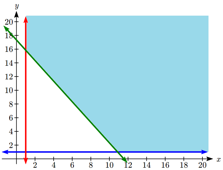
The region is unbounded, but we will be able to find a minimum still. We can see there are two corner points.
The one in the upper left is the intersection of the lines ![]() and
and ![]() . Solving for the intersection using substitution:
. Solving for the intersection using substitution:
![]()
Point: ![]()
The one in the lower right is the intersection of the lines ![]() and
and ![]() .
.
![]()
Point: ![]()
Testing the objective function at each of these corner points:
| Point | Cost, |
The company can minimize cost by using 1 serving of apricots and 15.8 servings of dates.
Give It Some Thought
2. A company makes two products. Product A requires 3 hours of manufacturing and 1 hour of assembly. Product B requires 4 hours of manufacturing and 2 hours of assembly. There are a total of 84 hours of manufacturing and 32 hours of assembly available. Determine the production to maximize profit if the profit on product A is $50 and the profit on product B is $60.
Example 8.4C
A factory manufactures chairs and tables, each requiring the use of three operations: Cutting, Assembly, and Finishing. The first operation can be used at most 40 hours; the second at most 42 hours; and the third at most 25 hours. A chair requires 1 hour of cutting, 2 hours of assembly, and 1 hour of finishing; a table needs 2 hours of cutting, 1 hour of assembly, and 1 hour of finishing. If the profit is $20 per unit for a chair and $30 for a table, how many units of each should be manufactured to maximize profit?
We begin by defining the variables. Let
![]() = number of chairs made
= number of chairs made
![]() = number of tables made
= number of tables made
The profit, ![]() , will be
, will be ![]() .
.
For cutting, ![]() chairs will require
chairs will require ![]() hours and
hours and ![]() tables will require
tables will require ![]() hours. We can use at most 40 hours, so
hours. We can use at most 40 hours, so ![]() .
.
For assembly, ![]() chairs will require
chairs will require ![]() hours and
hours and ![]() tables will require
tables will require ![]() hours. We can use at most 42 hours, so
hours. We can use at most 42 hours, so ![]() .
.
For finishing, ![]() chairs will require
chairs will require ![]() hours and
hours and ![]() tables will require
tables will require ![]() hours. We can use at most 25 hours, so
hours. We can use at most 25 hours, so ![]() .
.
Since we can’t produce negative items, ![]() .
.
Graphing the constraints, we can see the feasible region.
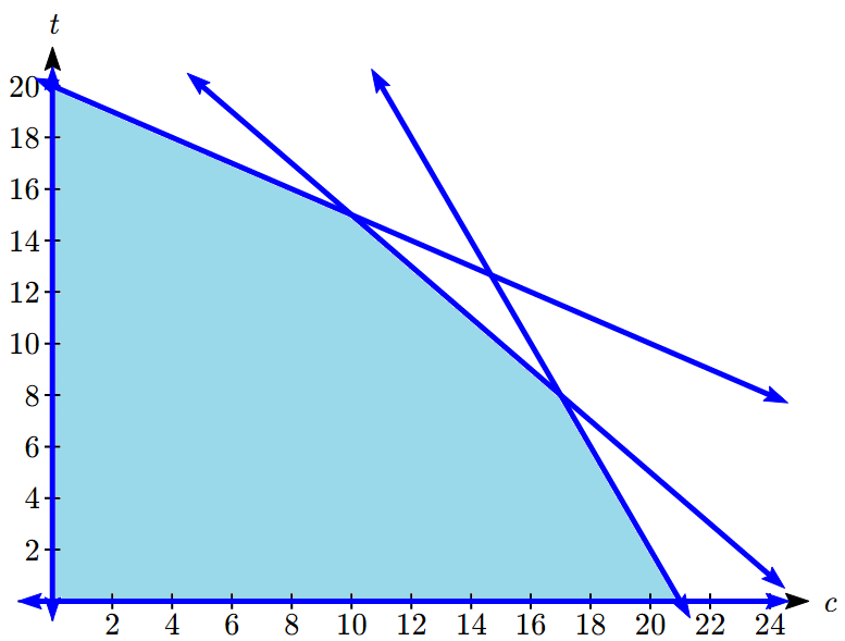
There are five corner points for this region.
Point 1: In the lower left, where ![]() crosses
crosses ![]() .
.
Point: ![]()
Point 2: In the upper left, where ![]() crosses
crosses ![]() .
.
Using substitution, ![]() , so
, so ![]() .
.
Point: ![]()
Point 3: In the lower right, where ![]() crosses
crosses ![]() .
.
Using substitution, ![]() , so
, so ![]() .
.
Point: ![]()
Point 4: Where ![]() crosses
crosses ![]() .
.
We can solve this as a system using any techniques we know. We could solve the second equation for ![]() , giving
, giving ![]() , then substitute into the first equation:
, then substitute into the first equation:

Then ![]() .
.
Point: ![]()
Point 5: Where ![]() crosses
crosses ![]() .
.
We can solve this as a system using any techniques we know. Using a different technique this time, we could multiply the bottom equation by -1 then add it to the first:

Then using ![]() , we have
, we have ![]() , so
, so ![]() .
.
Point: ![]()
Testing the objective function at each of these corner points:
| Point | Profit, |
The profit will be maximized by producing 10 chairs and 15 tables.
Give It Some Thought Answers
1. Maximize ![]() subject to:
subject to:

Graphing the feasible region, we see there are three corner points of potential interest: ![]() ,
, ![]() , and the intersection of the two lines at
, and the intersection of the two lines at ![]() . We then evaluate the objective function at each corner point.
. We then evaluate the objective function at each corner point.
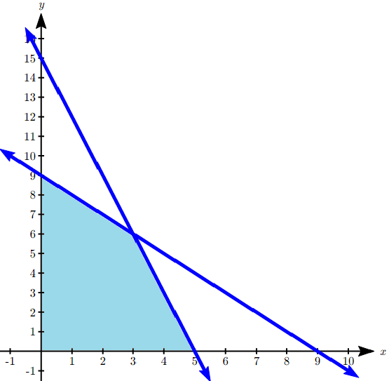
| Point | |
| 81 | |
| 70 |
![]() is maximized when
is maximized when ![]() ,
, ![]() .
.
2. Let ![]() be the number of product A produced, and
be the number of product A produced, and ![]() be the number of product B.
be the number of product B.
Our goal is to maximize profit: ![]() .
.
From manufacturing we get the constraint:
![]()
From assembly we get the constraint:
![]()
We have corner points at (0, 16), (28, 0). The third is at the intersection of the two lines. To find that we could multiply the second equation by -2 and add:

The third corner point is at ![]() .
.

Evaluating the objective function at each of these points:
| Point | |
Profit will be maximized by producing 28 units of product A and 0 units of product B.
Section 8.4 Exercises
Insert review exercises here
Chapter 8 Summary
Key Takeaways
Section 8.1: Systems of Equations
- Solving systems
Graphing
Elimination
Addition - Setting up systems of equations
- Inconsistent and dependent systems
- Solving 3 by 3 systems
Section 8.2: Inequalities in One Variable
- The properties of the absolute value function
- Solving absolute value equations
- Finding intercepts
- Solving absolute value inequalities
Section 8.3: Linear Inequalities
- Graphing linear inequalities
Dashed line for strict inequalities, solid for ≤ or ≥ - Graphing systems of linear inequalities
Section 8.4: Graphical Solutions
- Objective function
- Constraint equations
- Feasible region
- Corner points
- Fundamental Theorem of Linear Programming
- Solving a linear programming problem using a graph
- http://www.pollingreport.com/civil.htm, retrieved August 4, 2010 ↵
- Technically, margin of error usually means that the surveyors are 95% confident that actual value falls within this range. ↵
A set of two or more equations made up of two or more variables such that all equations in the system are considered simultaneously; the solution is a set of numerical values for each variable in the system that will satisfy all the equations in the system at the same time
A system of equations that has at least one solution
A consistent system in which the equations represent lines that intersect only once; has exactly one solution
A consistent system in which the equations represent the same line; has infinite solutions
A system of equations in which the equations represent two parallel lines; has no solution
A function whose value we either want to be as large as possible (want to maximize it) or as small as possible (want to minimize it)
The set of possible solutions to a system as shown on a graph

