5 Statistical Thinking
Original chapter by Beth Chance and Allan Rossman adapted by the Queen’s University Psychology Department
This Open Access chapter was originally written for the NOBA project. Information on the NOBA project can be found below.
We encourage students to use the “Three-Step Method” for support in their learning. Please find our version of the Three-Step Method, created in collaboration with Queen’s Student Academic Success Services, at the following link: https://sass.queensu.ca/psyc100/
As our society increasingly calls for evidence-based decision making, it is important to consider how and when we can draw valid inferences from data. This module will use four recent research studies to highlight key elements of a statistical investigation.
Learning Objectives
- Define basic elements of a statistical investigation.
- Describe the role of p-values and confidence intervals in statistical inference.
- Describe the role of random sampling in generalizing conclusions from a sample to a population.
- Describe the role of random assignment in drawing cause-and-effect conclusions.
- Critique statistical studies.
Introduction
Does drinking coffee actually increase your life expectancy? A recent study (Freedman, Park, Abnet, Hollenbeck, & Sinha, 2012) found that men who drank at least six cups of coffee a day had a 10% lower chance of dying (women 15% lower) than those who drank none. Does this mean you should pick up or increase your own coffee habit?
Modern society has become awash in studies such as this; you can read about several such studies in the news every day. Moreover, data abound everywhere in modern life. Conducting such a study well, and interpreting the results of such studies well for making informed decisions or setting policies, requires understanding basic ideas of statistics, the science of gaining insight from data. Rather than relying on anecdote and intuition, statistics allows us to systematically study phenomena of interest.

Key components to a statistical investigation are:
- Planning the study: Start by asking a testable research question and deciding how to collect data. For example, how long was the study period of the coffee study? How many people were recruited for the study, how were they recruited, and from where? How old were they? What other variables were recorded about the individuals, such as smoking habits, on the comprehensive lifestyle questionnaires? Were changes made to the participants’ coffee habits during the course of the study?
- Examining the data: What are appropriate ways to examine the data? What graphs are relevant, and what do they reveal? What descriptive statistics can be calculated to summarize relevant aspects of the data, and what do they reveal? What patterns do you see in the data? Are there any individual observations that deviate from the overall pattern, and what do they reveal? For example, in the coffee study, did the proportions differ when we compared the smokers to the non-smokers? Is there evidence for reliability and validity?
- Inferring from the data: What are valid statistical methods for drawing inferences “beyond” the data you collected? In the coffee study, is the 10%–15% reduction in risk of death something that could have happened just by chance?
- Drawing conclusions: Based on what you learned from your data, what conclusions can you draw? Who do you think these conclusions apply to? (Were the people in the coffee study older? Healthy? Living in cities?) Can you draw a cause-and-effect conclusion about your treatments? (Are scientists now saying that the coffee drinking is the cause of the decreased risk of death?)
Notice that the numerical analysis (“crunching numbers” on the computer) comprises only a small part of overall statistical investigation. In this module, you will see how we can answer some of these questions and what questions you should be asking about any statistical investigation you read about.
Distributional Thinking
When data are collected to address a particular question, an important first step is to think of meaningful ways to organize and examine the data. The most fundamental principle of statistics is that data vary. The pattern of that variation is crucial to capture and to understand. Often, careful presentation of the data will address many of the research questions without requiring more sophisticated analyses. It may, however, point to additional questions that need to be examined in more detail.
Example 1: Researchers investigated whether cancer pamphlets are written at an appropriate level to be read and understood by cancer patients (Short, Moriarty, & Cooley, 1995). Tests of reading ability were given to 63 patients. In addition, readability level was determined for a sample of 30 pamphlets, based on characteristics such as the lengths of words and sentences in the pamphlet. The results, reported in terms of grade levels, are displayed in Table 1.
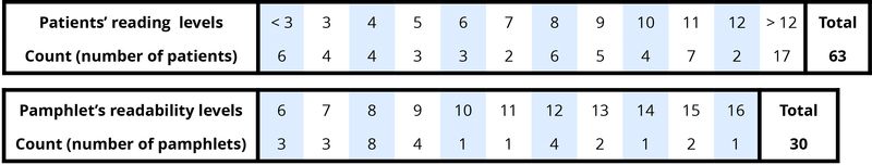
These two variables reveal two fundamental aspects of statistical thinking:
- Data vary. More specifically, values of a variable (such as reading level of a cancer patient or readability level of a cancer pamphlet) vary.
- Analyzing the pattern of variation, called the distribution of the variable, often reveals insights.
Addressing the research question of whether the cancer pamphlets are written at appropriate levels for the cancer patients requires comparing the two distributions. A naïve comparison might focus only on the centers of the distributions. Both medians turn out to be ninth grade, but considering only medians ignores the variability and the overall distributions of these data. A more illuminating approach is to compare the entire distributions, for example with a graph, as in Figure 1.
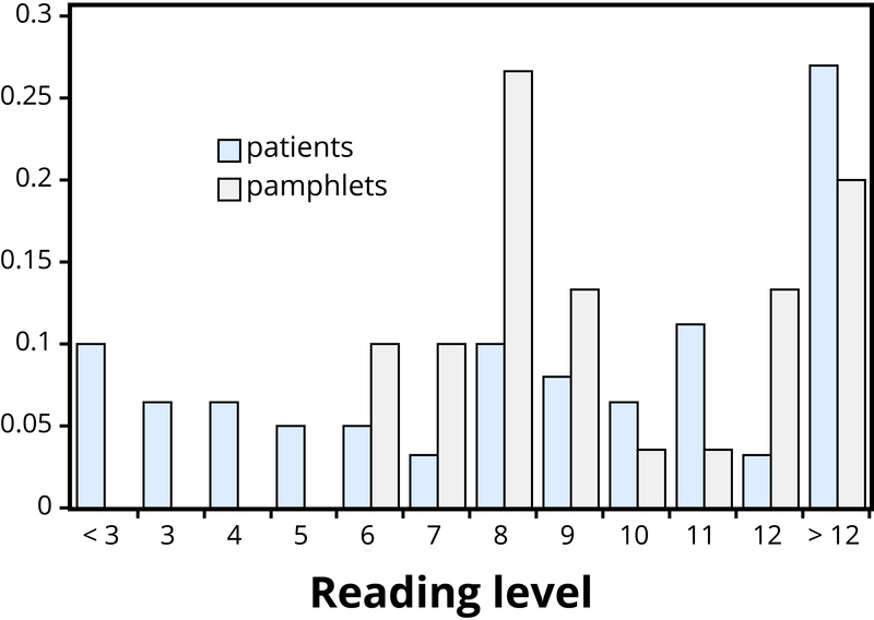
Figure 1 makes clear that the two distributions are not well aligned at all. The most glaring discrepancy is that many patients (17/63, or 27%, to be precise) have a reading level below that of the most readable pamphlet. These patients will need help to understand the information provided in the cancer pamphlets. Notice that this conclusion follows from considering the distributions as a whole, not simply measures of center or variability, and that the graph contrasts those distributions more immediately than the frequency tables.
Statistical Significance
Even when we find patterns in data, often there is still uncertainty in various aspects of the data. For example, there may be potential for measurement errors (even your own body temperature can fluctuate by almost 1 °F over the course of the day). Or we may only have a “snapshot” of observations from a more long-term process or only a small subset of individuals from the population of interest. In such cases, how can we determine whether patterns we see in our small set of data is convincing evidence of a systematic phenomenon in the larger process or population?
Example 2: In a study reported in the November 2007 issue of Nature, researchers investigated whether pre-verbal infants take into account an individual’s actions toward others in evaluating that individual as appealing or aversive (Hamlin, Wynn, & Bloom, 2007). In one component of the study, 10-month-old infants were shown a “climber” character (a piece of wood with “googly” eyes glued onto it) that could not make it up a hill in two tries. Then the infants were shown two scenarios for the climber’s next try, one where the climber was pushed to the top of the hill by another character (“helper”), and one where the climber was pushed back down the hill by another character (“hinderer”). The infant was alternately shown these two scenarios several times. Then the infant was presented with two pieces of wood (representing the helper and the hinderer characters) and asked to pick one to play with. The researchers found that of the 16 infants who made a clear choice, 14 chose to play with the helper toy.

One possible explanation for this clear majority result is that the helping behavior of the one toy increases the infants’ likelihood of choosing that toy. But are there other possible explanations? What about the color of the toy? Well, prior to collecting the data, the researchers arranged so that each color and shape (red square and blue circle) would be seen by the same number of infants. Or maybe the infants had right-handed tendencies and so picked whichever toy was closer to their right hand? Well, prior to collecting the data, the researchers arranged it so half the infants saw the helper toy on the right and half on the left. Or, maybe the shapes of these wooden characters (square, triangle, circle) had an effect? Perhaps, but again, the researchers controlled for this by rotating which shape was the helper toy, the hinderer toy, and the climber. When designing experiments, it is important to control for as many variables as might affect the responses as possible.
It is beginning to appear that the researchers accounted for all the other plausible explanations. But there is one more important consideration that cannot be controlled—if we did the study again with these 16 infants, they might not make the same choices. In other words, there is some randomness inherent in their selection process. Maybe each infant had no genuine preference at all, and it was simply “random luck” that led to 14 infants picking the helper toy. Although this random component cannot be controlled, we can apply a probability model to investigate the pattern of results that would occur in the long run if random chance were the only factor.
If the infants were equally likely to pick between the two toys, then each infant had a 50% chance of picking the helper toy. It’s like each infant tossed a coin, and if it landed heads, the infant picked the helper toy. So if we tossed a coin 16 times, could it land heads 14 times? Sure, it’s possible, but it turns out to be very unlikely. Getting 14 (or more) heads in 16 tosses is about as likely as tossing a coin and getting 9 heads in a row. This probability is referred to as a p-value. The p-value tells you how often a random process would give a result at least as extreme as what was found in the actual study, assuming there was nothing other than random chance at play. So, if we assume that each infant was choosing equally, then the probability that 14 or more out of 16 infants would choose the helper toy is found to be 0.0021. We have only two logical possibilities: either the infants have a genuine preference for the helper toy, or the infants have no preference (50/50) and an outcome that would occur only 2 times in 1,000 iterations happened in this study. Because this p-value of 0.0021 is quite small, we conclude that the study provides very strong evidence that these infants have a genuine preference for the helper toy. We often compare the p-value to some cut-off value (called the level of significance, typically around 0.05). If the p-value is smaller than that cut-off value, then we reject the hypothesis that only random chance was at play here. In this case, these researchers would conclude that significantly more than half of the infants in the study chose the helper toy, giving strong evidence of a genuine preference for the toy with the helping behavior.
Generalizability

One limitation to the previous study is that the conclusion only applies to the 16 infants in the study. We don’t know much about how those 16 infants were selected. Suppose we want to select a subset of individuals (a sample) from a much larger group of individuals (the population) in such a way that conclusions from the sample can be generalized to the larger population. This is the question faced by pollsters every day.
Example 3: The General Social Survey (GSS) is a survey on societal trends conducted every other year in the United States. Based on a sample of about 2,000 adult Americans, researchers make claims about what percentage of the U.S. population consider themselves to be “liberal,” what percentage consider themselves “happy,” what percentage feel “rushed” in their daily lives, and many other issues. The key to making these claims about the larger population of all American adults lies in how the sample is selected. The goal is to select a sample that is representative of the population, and a common way to achieve this goal is to select a random sample that gives every member of the population an equal chance of being selected for the sample. In its simplest form, random sampling involves numbering every member of the population and then using a computer to randomly select the subset to be surveyed. Most polls don’t operate exactly like this, but they do use probability-based sampling methods to select individuals from nationally representative panels.
In 2004, the GSS reported that 817 of 977 respondents (or 83.6%) indicated that they always or sometimes feel rushed. This is a clear majority, but we again need to consider variation due to random sampling. Fortunately, we can use the same probability model we did in the previous example to investigate the probable size of this error. (Note, we can use the coin-tossing model when the actual population size is much, much larger than the sample size, as then we can still consider the probability to be the same for every individual in the sample.) This probability model predicts that the sample result will be within 3 percentage points of the population value (roughly 1 over the square root of the sample size, the margin of error). A statistician would conclude, with 95% confidence, that between 80.6% and 86.6% of all adult Americans in 2004 would have responded that they sometimes or always feel rushed.
The key to the margin of error is that when we use a probability sampling method, we can make claims about how often (in the long run, with repeated random sampling) the sample result would fall within a certain distance from the unknown population value by chance (meaning by random sampling variation) alone. Conversely, non-random samples are often suspect to bias, meaning the sampling method systematically over-represents some segments of the population and under-represents others. We also still need to consider other sources of bias, such as individuals not responding honestly. These sources of error are not measured by the margin of error.
Cause and Effect Conclusions
In many research studies, the primary question of interest concerns differences between groups. Then the question becomes how were the groups formed (e.g., selecting people who already drink coffee vs. those who don’t). In some studies, the researchers actively form the groups themselves. But then we have a similar question—could any differences we observe in the groups be an artifact of that group-formation process? Or maybe the difference we observe in the groups is so large that we can discount a “fluke” in the group-formation process as a reasonable explanation for what we find?
Example 4: A psychology study investigated whether people tend to display more creativity when they are thinking about intrinsic or extrinsic motivations (Ramsey & Schafer, 2002, based on a study by Amabile, 1985). The subjects were 47 people with extensive experience with creative writing. Subjects began by answering survey questions about either intrinsic motivations for writing (such as the pleasure of self-expression) or extrinsic motivations (such as public recognition). Then all subjects were instructed to write a haiku, and those poems were evaluated for creativity by a panel of judges. The researchers conjectured beforehand that subjects who were thinking about intrinsic motivations would display more creativity than subjects who were thinking about extrinsic motivations. The creativity scores from the 47 subjects in this study are displayed in Figure 2, where higher scores indicate more creativity.
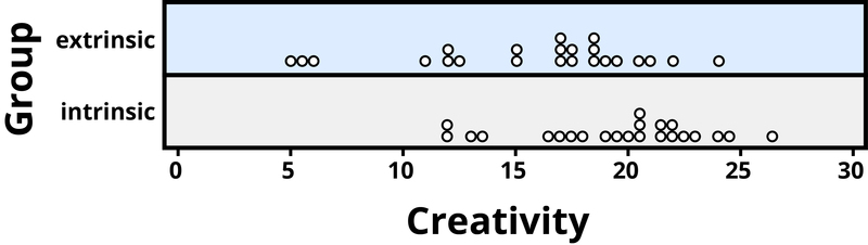
In this example, the key question is whether the type of motivation affects creativity scores. In particular, do subjects who were asked about intrinsic motivations tend to have higher creativity scores than subjects who were asked about extrinsic motivations?
Figure 2 reveals that both motivation groups saw considerable variability in creativity scores, and these scores have considerable overlap between the groups. In other words, it’s certainly not always the case that those with extrinsic motivations have higher creativity than those with intrinsic motivations, but there may still be a statistical tendency in this direction. (Psychologist Keith Stanovich (2013) refers to people’s difficulties with thinking about such probabilistic tendencies as “the Achilles heel of human cognition.”)
The mean creativity score is 19.88 for the intrinsic group, compared to 15.74 for the extrinsic group, which supports the researchers’ conjecture. Yet comparing only the means of the two groups fails to consider the variability of creativity scores in the groups. We can measure variability with statistics using, for instance, the standard deviation: 5.25 for the extrinsic group and 4.40 for the intrinsic group. The standard deviations tell us that most of the creativity scores are within about 5 points of the mean score in each group. We see that the mean score for the intrinsic group lies within one standard deviation of the mean score for extrinsic group. So, although there is a tendency for the creativity scores to be higher in the intrinsic group, on average, the difference is not extremely large.
We again want to consider possible explanations for this difference. The study only involved individuals with extensive creative writing experience. Although this limits the population to which we can generalize, it does not explain why the mean creativity score was a bit larger for the intrinsic group than for the extrinsic group. Maybe women tend to receive higher creativity scores? Here is where we need to focus on how the individuals were assigned to the motivation groups. If only women were in the intrinsic motivation group and only men in the extrinsic group, then this would present a problem because we wouldn’t know if the intrinsic group did better because of the different type of motivation or because they were women. However, the researchers guarded against such a problem by randomly assigning the individuals to the motivation groups. Like flipping a coin, each individual was just as likely to be assigned to either type of motivation. Why is this helpful? Because this random assignment tends to balance out all the variables related to creativity we can think of, and even those we don’t think of in advance, between the two groups. So we should have a similar male/female split between the two groups; we should have a similar age distribution between the two groups; we should have a similar distribution of educational background between the two groups; and so on. Random assignment should produce groups that are as similar as possible except for the type of motivation, which presumably eliminates all those other variables as possible explanations for the observed tendency for higher scores in the intrinsic group.
But does this always work? No, so by “luck of the draw” the groups may be a little different prior to answering the motivation survey. So then the question is, is it possible that an unlucky random assignment is responsible for the observed difference in creativity scores between the groups? In other words, suppose each individual’s poem was going to get the same creativity score no matter which group they were assigned to, that the type of motivation in no way impacted their score. Then how often would the random-assignment process alone lead to a difference in mean creativity scores as large (or larger) than 19.88 – 15.74 = 4.14 points?
We again want to apply to a probability model to approximate a p-value, but this time the model will be a bit different. Think of writing everyone’s creativity scores on an index card, shuffling up the index cards, and then dealing out 23 to the extrinsic motivation group and 24 to the intrinsic motivation group, and finding the difference in the group means. We (better yet, the computer) can repeat this process over and over to see how often, when the scores don’t change, random assignment leads to a difference in means at least as large as 4.41. Figure 3 shows the results from 1,000 such hypothetical random assignments for these scores.
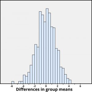
Only 2 of the 1,000 simulated random assignments produced a difference in group means of 4.41 or larger. In other words, the approximate p-value is 2/1000 = 0.002. This small p-value indicates that it would be very surprising for the random assignment process alone to produce such a large difference in group means. Therefore, as with Example 2, we have strong evidence that focusing on intrinsic motivations tends to increase creativity scores, as compared to thinking about extrinsic motivations.
Notice that the previous statement implies a cause-and-effect relationship between motivation and creativity score; is such a strong conclusion justified? Yes, because of the random assignment used in the study. That should have balanced out any other variables between the two groups, so now that the small p-value convinces us that the higher mean in the intrinsic group wasn’t just a coincidence, the only reasonable explanation left is the difference in the type of motivation. Can we generalize this conclusion to everyone? Not necessarily—we could cautiously generalize this conclusion to individuals with extensive experience in creative writing similar the individuals in this study, but we would still want to know more about how these individuals were selected to participate.
The Importance of Diversity in Psychological Science
It is critically important that we carefully consider the extent to which our samples are truly diverse and random, the possibilities for alternative explanations for our results, and the degree to which our findings may (or may not) be generalizable. For example, historically, psychological science (and in science more broadly), has commonly used dichotomous categories of “men” and “women” to compare and contrast patterns of results. It is not always clear the degree to which these dichotomous terms have assessed sex, gender, or both. Further, this dichotomy of “men” and “women” (“male and “female,” etc.) fails to include many people who may not identify in a binary manner. Thus, it could be that there are limitations with interpretation of some of these findings. The topic of sex and gender can be considered as a lens for research, but also as its own major topic area in Psychology. For this reason, we will cover the topic of sex and gender in detail in our unit related to self and identity. We want to highlight this topic for your consideration here, and also link you to that chapter now if you would like to consider it in more detail earlier in our content.
Just as considering diversity related to sex and gender is important, so is considering diversity more broadly. For example, factors including (but not limited to) race, age, geographic location, socioeconomic status, and more, can have important influences on many research questions. We will highlight the need for diversity and inclusion in psychological science throughout our course, and encourage you to continually question the degree to which our science can be more inclusive and diverse.
Conclusion

Statistical thinking involves the careful design of a study to collect meaningful data to answer a focused research question, detailed analysis of patterns in the data, and drawing conclusions that go beyond the observed data. Random sampling is paramount to generalizing results from our sample to a larger population, and random assignment is key to drawing cause-and-effect conclusions. With both kinds of randomness, probability models help us assess how much random variation we can expect in our results, in order to determine whether our results could happen by chance alone and to estimate a margin of error.
So where does this leave us with regard to the coffee study mentioned at the beginning of this module? We can answer many of the questions:
- This was a 14-year study conducted by researchers at the National Cancer Institute.
- The results were published in the June issue of the New England Journal of Medicine, a respected, peer-reviewed journal.
- The study reviewed coffee habits of more than 402,000 people ages 50 to 71 from six states and two metropolitan areas. Those with cancer, heart disease, and stroke were excluded at the start of the study. Coffee consumption was assessed once at the start of the study.
- About 52,000 people died during the course of the study.
- People who drank between two and five cups of coffee daily showed a lower risk as well, but the amount of reduction increased for those drinking six or more cups.
- The sample sizes were fairly large and so the p-values are quite small, even though percent reduction in risk was not extremely large (dropping from a 12% chance to about 10%–11%).
- Whether coffee was caffeinated or decaffeinated did not appear to affect the results.
- This was an observational study, so no cause-and-effect conclusions can be drawn between coffee drinking and increased longevity, contrary to the impression conveyed by many news headlines about this study. In particular, it’s possible that those with chronic diseases don’t tend to drink coffee.
This study needs to be reviewed in the larger context of similar studies and consistency of results across studies, with the constant caution that this was not a randomized experiment. Whereas a statistical analysis can still “adjust” for other potential confounding variables, we are not yet convinced that researchers have identified them all or completely isolated why this decrease in death risk is evident. Researchers can now take the findings of this study and develop more focused studies that address new questions.
Check Your Knowledge
To help you with your studying, we’ve included some practice questions for this module. These questions do not necessarily address all content in this module. They are intended as practice, and you are responsible for all of the content in this module even if there is no associated practice question. To promote deeper engagement with the material, we encourage you to create some questions of your own for your practice. You can then also return to these self-generated questions later in the course to test yourself.
Vocabulary
- Cause-and-effect
- Related to whether we say one variable is causing changes in the other variable, versus other variables that may be related to these two variables.
- Confidence interval
- An interval of plausible values for a population parameter; the interval of values within the margin of error of a statistic.
- Distribution
- The pattern of variation in data.
- Generalizability
- Related to whether the results from the sample can be generalized to a larger population.
- Margin of error
- The expected amount of random variation in a statistic; often defined for 95% confidence level.
- Parameter
- A numerical result summarizing a population (e.g., mean, proportion).
- Population
- A larger collection of individuals that we would like to generalize our results to.
- P-value
- The probability of observing a particular outcome in a sample, or more extreme, under a conjecture about the larger population or process.
- Random assignment
- Using a probability-based method to divide a sample into treatment groups.
- Random sampling
- Using a probability-based method to select a subset of individuals for the sample from the population.
- Reliability
- The consistency of a measure.
- Sample
- The collection of individuals on which we collect data.
- Statistic
- A numerical result computed from a sample (e.g., mean, proportion).
- Statistical significance
- A result is statistically significant if it is unlikely to arise by chance alone.
- Validity
- The degree to which a measure is assessing what it is intended to measure.
-
References
- Amabile, T. (1985). Motivation and creativity: Effects of motivational orientation on creative writers. Journal of Personality and Social Psychology, 48(2), 393–399.
- Freedman, N. D., Park, Y., Abnet, C. C., Hollenbeck, A. R., & Sinha, R. (2012). Association of coffee drinking with total and cause-specific mortality. New England Journal of Medicine, 366, 1891–1904.
- Hamlin, J. K., Wynn, K., & Bloom, P. (2007). Social evaluation by preverbal infants. Nature, 452(22), 557–560.
- Ramsey, F., & Schafer, D. (2002). The statistical sleuth: A course in methods of data analysis. Belmont, CA: Duxbury.
- Short, T., Moriarty, H., & Cooley, M. E. (1995). Readability of educational materials for patients with cancer. Journal of Statistics Education, 3(2).
- Stanovich, K. (2013). How to think straight about psychology (10th ed.). Upper Saddle River, NJ: Pearson.
How to cite this Chapter using APA Style:
Chance, B. & Rossman, A. (2019). Statistical thinking. Adapted for use by Queen’s University. Original chapter in R. Biswas-Diener & E. Diener (Eds), Noba textbook series: Psychology. Champaign, IL: DEF publishers. Retrieved from http://noba.to/ruaz6wjs
Copyright and Acknowledgment:
This material is licensed under the Creative Commons Attribution-NonCommercial-ShareAlike 4.0 International License. To view a copy of this license, visit: http://creativecommons.org/licenses/by-nc-sa/4.0/deed.en_US.
This material is attributed to the Diener Education Fund (copyright © 2018) and can be accessed via this link: http://noba.to/ruaz6wjs.
Additional information about the Diener Education Fund (DEF) can be accessed here.
Freedman, N. D., Park, Y., Abnet, C. C., Hollenbeck, A. R., & Sinha, R. (2012). Association of coffee drinking with total and cause-specific mortality. New England Journal of Medicine, 366, 1891–1904.
Reliability refers to the consistency of a measure
Validity is the degree to which a measure is assessing what it is intended to measure
Related to whether we say one variable is causing changes in the other variable, versus other variables that may be related to these two variables.
Short, T., Moriarty, H., & Cooley, M. E. (1995). Readability of educational materials for patients with cancer. Journal of Statistics Education, 3(2).
The pattern of variation in data.
Hamlin, J. K., Wynn, K., & Bloom, P. (2007). Social evaluation by preverbal infants. Nature, 452(22), 557–560.
The probability of observing a particular outcome in a sample, or more extreme, under a conjecture about the larger population or process.
A result is statistically significant if it is unlikely to arise by chance alone.
The collection of individuals on which we collect data.
A larger collection of individuals that we would like to generalize our results to.
Related to whether the results from the sample can be generalized to a larger population.
Using a probability-based method to select a subset of individuals for the sample from the population.
The expected amount of random variation in a statistic; often defined for 95% confidence level.
Ramsey, F., & Schafer, D. (2002). The statistical sleuth: A course in methods of data analysis. Belmont, CA: Duxbury.
Amabile, T. (1985). Motivation and creativity: Effects of motivational orientation on creative writers. Journal of Personality and Social Psychology, 48(2), 393–399.
Stanovich, K. (2013). How to think straight about psychology (10th ed.). Upper Saddle River, NJ: Pearson.
Using a probability-based method to divide a sample into treatment groups.
