Chapter 7.2: The Central Limit Theorem for Sample Means (Averages)
Suppose X is a random variable with a distribution that may be known or unknown (it can be any distribution). Using a subscript that matches the random variable, suppose:
- μX = the mean of X
- σX = the standard deviation of X
If you draw random samples of size n, then as n increases, the random variable ![]() which consists of sample means, tends to be normally distributed and
which consists of sample means, tends to be normally distributed and
![]() ~ N
~ N![]() .
.
The central limit theorem for sample means says that if you keep drawing larger and larger samples (such as rolling one, two, five, and finally, ten dice) and calculating their means, the sample means form their own normal distribution (the sampling distribution). The normal distribution has the same mean as the original distribution and a variance that equals the original variance divided by the sample size. Standard deviation is the square root of variance, so the standard deviation of the sampling distribution is the standard deviation of the original distribution divided by the square root of n. The variable n is the number of values that are averaged together, not the number of times the experiment is done.
To put it more formally, if you draw random samples of size n, the distribution of the random variable ![]() , which consists of sample means, is called the sampling distribution of the mean. The sampling distribution of the mean approaches a normal distribution as n, the sample size, increases.
, which consists of sample means, is called the sampling distribution of the mean. The sampling distribution of the mean approaches a normal distribution as n, the sample size, increases.
The random variable ![]() has a different z-score associated with it from that of the random variable X. The mean
has a different z-score associated with it from that of the random variable X. The mean ![]() is the value of
is the value of ![]() in one sample.
in one sample.
μX is the average of both X and ![]() .
.
![]() = standard deviation of
= standard deviation of ![]() and is called the standard error of the mean.
and is called the standard error of the mean.
To find probabilities for means on the calculator, follow these steps.
2nd DISTR
2:normalcdf
![]()
where:
- mean is the mean of the original distribution
- standard deviation is the standard deviation of the original distribution
- sample size = n
An unknown distribution has a mean of 90 and a standard deviation of 15. Samples of size n = 25 are drawn randomly from the population.
a. Find the probability that the sample mean is between 85 and 92.
a. Let X = one value from the original unknown population. The probability question asks you to find a probability for the sample mean.
Let ![]() = the mean of a sample of size 25. Since μX = 90, σX = 15, and n = 25,
= the mean of a sample of size 25. Since μX = 90, σX = 15, and n = 25,
![]() ~ N
~ N![]() .
.
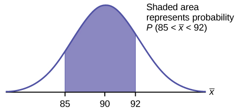
Find P(85 < ![]() < 92). Draw a graph.
< 92). Draw a graph.
P(85 < ![]() < 92) = 0.6997
< 92) = 0.6997
The probability that the sample mean is between 85 and 92 is 0.6997.

normalcdf(lower value, upper value, mean, standard error of the mean)
The parameter list is abbreviated (lower value, upper value, μ, ![]() )
)
normalcdf(85,92,90,![]() ) = 0.6997
) = 0.6997
b. Find the value that is two standard deviations above the expected value, 90, of the sample mean.
b. To find the value that is two standard deviations above the expected value 90, use the formula:
value = μx + (#ofTSDEVs)![]()
value = 90 + 2 ![]() = 96
= 96
The value that is two standard deviations above the expected value is 96.
The standard error of the mean is ![]() =
= ![]() = 3. Recall that the standard error of the mean is a description of how far (on average) that the sample mean will be from the population mean in repeated simple random samples of size n.
= 3. Recall that the standard error of the mean is a description of how far (on average) that the sample mean will be from the population mean in repeated simple random samples of size n.
An unknown distribution has a mean of 45 and a standard deviation of eight. Samples of size n = 30 are drawn randomly from the population. Find the probability that the sample mean is between 42 and 50.
The length of time, in hours, it takes an “over 40” group of people to play one soccer match is normally distributed with a mean of two hours and a standard deviation of 0.5 hours. A sample of size n = 50 is drawn randomly from the population. Find the probability that the sample mean is between 1.8 hours and 2.3 hours.
Let X = the time, in hours, it takes to play one soccer match.
The probability question asks you to find a probability for the sample mean time, in hours, it takes to play one soccer match.
Let ![]() = the mean time, in hours, it takes to play one soccer match.
= the mean time, in hours, it takes to play one soccer match.
If μX = _________, σX = __________, and n = ___________, then X ~ N(______, ______) by the central limit theorem for means.
μX = 2, σX = 0.5, n = 50, and X ~ N![]()
Find P(1.8 < ![]() < 2.3). Draw a graph.
< 2.3). Draw a graph.
P(1.8 < ![]() < 2.3) = 0.9977
< 2.3) = 0.9977
normalcdf![]() = 0.9977
= 0.9977
The probability that the mean time is between 1.8 hours and 2.3 hours is 0.9977.
The length of time taken on the SAT for a group of students is normally distributed with a mean of 2.5 hours and a standard deviation of 0.25 hours. A sample size of n = 60 is drawn randomly from the population. Find the probability that the sample mean is between two hours and three hours.
To find percentiles for means on the calculator, follow these steps.
2nd DIStR
3:invNorm
k = invNorm![]()
where:
- k = the kth percentile
- mean is the mean of the original distribution
- standard deviation is the standard deviation of the original distribution
- sample size = n
In a recent study reported Oct. 29, 2012 on the Flurry Blog, the mean age of tablet users is 34 years. Suppose the standard deviation is 15 years. Take a sample of size n = 100.
- What are the mean and standard deviation for the sample mean ages of tablet users?
- What does the distribution look like?
- Find the probability that the sample mean age is more than 30 years (the reported mean age of tablet users in this particular study).
- Find the 95th percentile for the sample mean age (to one decimal place).
- Since the sample mean tends to target the population mean, we have μχ = μ = 34. The sample standard deviation is given by σχ =
 =
=  =
=  = 1.5
= 1.5 - The central limit theorem states that for large sample sizes(n), the sampling distribution will be approximately normal.
- The probability that the sample mean age is more than 30 is given by P(Χ > 30) =
normalcdf(30,E99,34,1.5) = 0.9962 - Let k = the 95th percentile.
k = invNorm = 36.5
In an article on Flurry Blog, a gaming marketing gap for men between the ages of 30 and 40 is identified. You are researching a startup game targeted at the 35-year-old demographic. Your idea is to develop a strategy game that can be played by men from their late 20s through their late 30s. Based on the article’s data, industry research shows that the average strategy player is 28 years old with a standard deviation of 4.8 years. You take a sample of 100 randomly selected gamers. If your target market is 29- to 35-year-olds, should you continue with your development strategy?
The mean number of minutes for app engagement by a tablet user is 8.2 minutes. Suppose the standard deviation is one minute. Take a sample of 60.
- What are the mean and standard deviation for the sample mean number of app engagement by a tablet user?
- What is the standard error of the mean?
- Find the 90th percentile for the sample mean time for app engagement for a tablet user. Interpret this value in a complete sentence.
- Find the probability that the sample mean is between eight minutes and 8.5 minutes.
Cans of a cola beverage claim to contain 16 ounces. The amounts in a sample are measured and the statistics are n = 34, ![]() = 16.01 ounces. If the cans are filled so that μ = 16.00 ounces (as labeled) and σ = 0.143 ounces, find the probability that a sample of 34 cans will have an average amount greater than 16.01 ounces. Do the results suggest that cans are filled with an amount greater than 16 ounces?
= 16.01 ounces. If the cans are filled so that μ = 16.00 ounces (as labeled) and σ = 0.143 ounces, find the probability that a sample of 34 cans will have an average amount greater than 16.01 ounces. Do the results suggest that cans are filled with an amount greater than 16 ounces?
References
Baran, Daya. “20 Percent of Americans Have Never Used Email.”WebGuild, 2010. Available online at http://www.webguild.org/20080519/20-percent-of-americans-have-never-used-email (accessed May 17, 2013).
Data from The Flurry Blog, 2013. Available online at http://blog.flurry.com (accessed May 17, 2013).
Data from the United States Department of Agriculture.
Chapter Review
In a population whose distribution may be known or unknown, if the size (n) of samples is sufficiently large, the distribution of the sample means will be approximately normal. The mean of the sample means will equal the population mean. The standard deviation of the distribution of the sample means, called the standard error of the mean, is equal to the population standard deviation divided by the square root of the sample size (n).
Formula Review
The Central Limit Theorem for Sample Means: ![]() ~ N
~ N![]()
The Mean ![]() : μx
: μx
Central Limit Theorem for Sample Means z-score and standard error of the mean: ![]()
Standard Error of the Mean (Standard Deviation (![]() )):
)): ![]()
Use the following information to answer the next six exercises: Yoonie is a personnel manager in a large corporation. Each month she must review 16 of the employees. From past experience, she has found that the reviews take her approximately four hours each to do with a population standard deviation of 1.2 hours. Let Χ be the random variable representing the time it takes her to complete one review. Assume Χ is normally distributed. Let ![]() be the random variable representing the mean time to complete the 16 reviews. Assume that the 16 reviews represent a random set of reviews.
be the random variable representing the mean time to complete the 16 reviews. Assume that the 16 reviews represent a random set of reviews.
What is the mean, standard deviation, and sample size?
mean = 4 hours; standard deviation = 1.2 hours; sample size = 16
Complete the distributions.
- X ~ _____(_____,_____)
 ~ _____(_____,_____)
solution X ~ N(4, 1.2). X ¯ ~ N ( 4, 1.2 16 ) –>
Find the probability that one review will take Yoonie from 3.5 to 4.25 hours. Sketch the graph, labeling and scaling the horizontal axis. Shade the region corresponding to the probability.
-

- P(________ < x < ________) = _______
a. Check student’s solution.
b. 3.5, 4.25, 0.2441
Find the probability that the mean of a month’s reviews will take Yoonie from 3.5 to 4.25 hrs. Sketch the graph, labeling and scaling the horizontal axis. Shade the region corresponding to the probability.
-

- P(________________) = _______
solution b. 0.7499 –>
The fact that the two distributions are different accounts for the different probabilities.
Find the 95th percentile for the mean time to complete one month’s reviews. Sketch the graph.
-

- The 95th Percentile =____________
solution P(3.5 < x ¯ < 4.25) = invNorm ( 95,4, 1.2 16 ) = 4.49 –>
Homework
1) Previously, De Anza statistics students estimated that the amount of change daytime statistics students carry is exponentially distributed with a mean of $0.88. Suppose that we randomly pick 25 daytime statistics students.
- In words, Χ = ____________
- Χ ~ _____(_____,_____)
- In words,
 = ____________
  ~ ______ (______, ______)
- Find the probability that an individual had between $0.80 and $1.00. Graph the situation, and shade in the area to be determined.
- Find the probability that the average of the 25 students was between $0.80 and $1.00. Graph the situation, and shade in the area to be determined.
- Explain why there is a difference in part e and part f.
2) Suppose that the distance of fly balls hit to the outfield (in baseball) is normally distributed with a mean of 250 feet and a standard deviation of 50 feet. We randomly sample 49 fly balls.
- If
 = average distance in feet for 49 fly balls, then
  ~ _______(_______,_______)
 - What is the probability that the 49 balls traveled an average of less than 240 feet? Sketch the graph. Scale the horizontal axis for
 . Shade the region corresponding to the probability. Find the probability.
 - Find the 80th percentile of the distribution of the average of 49 fly balls.
3) According to the Internal Revenue Service, the average length of time for an individual to complete (keep records for, learn, prepare, copy, assemble, and send) IRS Form 1040 is 10.53 hours (without any attached schedules). The distribution is unknown. Let us assume that the standard deviation is two hours. Suppose we randomly sample 36 taxpayers.
- In words, Χ = _____________
- In words,
 = _____________
  ~ _____(_____,_____)
- Would you be surprised if the 36 taxpayers finished their Form 1040s in an average of more than 12 hours? Explain why or why not in complete sentences.
- Would you be surprised if one taxpayer finished his or her Form 1040 in more than 12 hours? In a complete sentence, explain why.
4) Suppose that a category of world-class runners are known to run a marathon (26 miles) in an average of 145 minutes with a standard deviation of 14 minutes. Consider 49 of the races. Let ![]() the average of the 49 races.
the average of the 49 races.
 ~ _____(_____,_____)
- Find the probability that the runner will average between 142 and 146 minutes in these 49 marathons.
- Find the 80th percentile for the average of these 49 marathons.
- Find the median of the average running times.
solution N ( 145, 14 49 ) 0.6247 146.68 145 minutes –>
5) The length of songs in a collector’s iTunes album collection is uniformly distributed from two to 3.5 minutes. Suppose we randomly pick five albums from the collection. There are a total of 43 songs on the five albums.
- In words, Χ = _________
- Χ ~ _____________
- In words,
 = _____________
  ~ _____(_____,_____)
- Find the first quartile for the average song length,
 .
. - The IQR (interquartile range) for the average song length,
 , is from ___ – ___.
6) In 1940 the average size of a U.S. farm was 174 acres. Let’s say that the standard deviation was 55 acres. Suppose we randomly survey 38 farmers from 1940.
- In words, Χ = _____________
- In words,
 = _____________
  ~ _____(_____,_____)
- The IQR for
 is from _______ acres to _______ acres.
7) Determine which of the following are true and which are false. Then, in complete sentences, justify your answers.
- When the sample size is large, the mean of
 is approximately equal to the mean of Χ.
 - When the sample size is large,
 is approximately normally distributed.
 - When the sample size is large, the standard deviation of
 is approximately the same as the standard deviation of Χ.
8) The percent of fat calories that a person in America consumes each day is normally distributed with a mean of about 36 and a standard deviation of about ten. Suppose that 16 individuals are randomly chosen. Let ![]() = average percent of fat calories.
= average percent of fat calories.
 ~ ______(______, ______)
- For the group of 16, find the probability that the average percent of fat calories consumed is more than five. Graph the situation and shade in the area to be determined.
- Find the first quartile for the average percent of fat calories.
9) The distribution of income in some Third World countries is considered wedge shaped (many very poor people, very few middle income people, and even fewer wealthy people). Suppose we pick a country with a wedge shaped distribution. Let the average salary be $2,000 per year with a standard deviation of $8,000. We randomly survey 1,000 residents of that country.
- In words, Χ = _____________
- In words,
 = _____________
  ~ _____(_____,_____)
- How is it possible for the standard deviation to be greater than the average?
- Why is it more likely that the average of the 1,000 residents will be from $2,000 to $2,100 than from $2,100 to $2,200?
10) Which of the following is NOT TRUE about the distribution for averages?
- The mean, median, and mode are equal.
- The area under the curve is one.
- The curve never touches the x-axis.
- The curve is skewed to the right.
11) The cost of unleaded gasoline in the Bay Area once followed an unknown distribution with a mean of $4.59 and a standard deviation of $0.10. Sixteen gas stations from the Bay Area are randomly chosen. We are interested in the average cost of gasoline for the 16 gas stations. The distribution to use for the average cost of gasoline for the 16 gas stations is:
 ~ N(4.59, 0.10)
 ~ N
~ N
 ~ N
~ N
 ~ N
~ N
Answers to odd questions
1)
- Χ = amount of change students carry
- Χ ~ E(0.88, 0.88)
 = average amount of change carried by a sample of 25 sstudents.
 ~ N(0.88, 0.176)
- 0.0819
- 0.1882
- The distributions are different. Part a is exponential and part b is normal.
3)
- length of time for an individual to complete IRS form 1040, in hours.
- mean length of time for a sample of 36 taxpayers to complete IRS form 1040, in hours.
- N

- Yes. I would be surprised, because the probability is almost 0.
- No. I would not be totally surprised because the probability is 0.2312
5)
- the length of a song, in minutes, in the collection
- U(2, 3.5)
- the average length, in minutes, of the songs from a sample of five albums from the collection
- N(2.75, 0.0660)
- 2.71 minutes
- 0.09 minutes
7)
- True. The mean of a sampling distribution of the means is approximately the mean of the data distribution.
- True. According to the Central Limit Theorem, the larger the sample, the closer the sampling distribution of the means becomes normal.
- The standard deviation of the sampling distribution of the means will decrease making it approximately the same as the standard deviation of X as the sample size increases.
9)
- X = the yearly income of someone in a third world country
- the average salary from samples of 1,000 residents of a third world country
 ∼ N
∼ N
- Very wide differences in data values can have averages smaller than standard deviations.
- The distribution of the sample mean will have higher probabilities closer to the population mean.
P(2000 < < 2100) = 0.1537
P(2100 < < 2200) = 0.1317
11) b
Glossary
- Average
- a number that describes the central tendency of the data; there are a number of specialized averages, including the arithmetic mean, weighted mean, median, mode, and geometric mean.
- Central Limit Theorem
- Given a random variable (RV) with known mean μ and known standard deviation, σ, we are sampling with size n, and we are interested in two new RVs: the sample mean,
 , and the sample sum, ΣΧ. If the size (n) of the sample is sufficiently large, then
  ~ N(μ,
  ) and ΣΧ ~ N(nμ, (
 )(σ)). If the size (n) of the sample is sufficiently large, then the distribution of the sample means and the distribution of the sample sums will approximate a normal distributions regardless of the shape of the population. The mean of the sample means will equal the population mean, and the mean of the sample sums will equal n times the population mean. The standard deviation of the distribution of the sample means,
  , is called the standard error of the mean.
- Normal Distribution
- a continuous random variable (RV) with pdf
 , where μ is the mean of the distribution and σ is the standard deviation; notation: Χ ~ N(μ, σ). If μ = 0 and σ = 1, the RV is called a standard normal distribution.
- Standard Error of the Mean
- the standard deviation of the distribution of the sample means, or
 .
.

