Chapter 11.3: Goodness-of-Fit Test
In this type of hypothesis test, you determine whether the data “fit” a particular distribution or not. For example, you may suspect your unknown data fit a binomial distribution. You use a chi-square test (meaning the distribution for the hypothesis test is chi-square) to determine if there is a fit or not. The null and the alternative hypotheses for this test may be written in sentences or may be stated as equations or inequalities.
The test statistic for a goodness-of-fit test is:

where:
- O = observed values (data)
- E = expected values (from theory)
- k = the number of different data cells or categories
The observed values are the data values and the expected values are the values you would expect to get if the null hypothesis were true. There are n terms of the form  .
.
The number of degrees of freedom is df = (number of categories – 1).
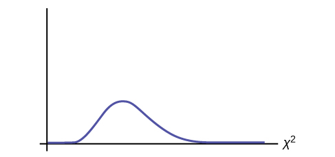
The goodness-of-fit test is almost always right-tailed. If the observed values and the corresponding expected values are not close to each other, then the test statistic can get very large and will be way out in the right tail of the chi-square curve.
The expected value for each cell needs to be at least five in order for you to use this test.
Absenteeism of college students from math classes is a major concern to math instructors because missing class appears to increase the drop rate. Suppose that a study was done to determine if the actual student absenteeism rate follows faculty perception. The faculty expected that a group of 100 students would miss class according to (Figure).
| Number of absences per term | Expected number of students |
|---|---|
| 0–2 | 50 |
| 3–5 | 30 |
| 6–8 | 12 |
| 9–11 | 6 |
| 12+ | 2 |
A random survey across all mathematics courses was then done to determine the actual number (observed) of absences in a course. The chart in (Figure) displays the results of that survey.
| Number of absences per term | Actual number of students |
|---|---|
| 0–2 | 35 |
| 3–5 | 40 |
| 6–8 | 20 |
| 9–11 | 1 |
| 12+ | 4 |
Determine the null and alternative hypotheses needed to conduct a goodness-of-fit test.
H0: Student absenteeism fits faculty perception.
The alternative hypothesis is the opposite of the null hypothesis.
Ha: Student absenteeism does not fit faculty perception.
a. Can you use the information as it appears in the charts to conduct the goodness-of-fit test?
a. No. Notice that the expected number of absences for the “12+” entry is less than five (it is two). Combine that group with the “9–11” group to create new tables where the number of students for each entry are at least five. The new results are in (Figure) and (Figure).
| Number of absences per term | Expected number of students |
|---|---|
| 0–2 | 50 |
| 3–5 | 30 |
| 6–8 | 12 |
| 9+ | 8 |
| Number of absences per term | Actual number of students |
|---|---|
| 0–2 | 35 |
| 3–5 | 40 |
| 6–8 | 20 |
| 9+ | 5 |
b. What is the number of degrees of freedom (df)?
b. There are four “cells” or categories in each of the new tables.
df = number of cells – 1 = 4 – 1 = 3
A factory manager needs to understand how many products are defective versus how many are produced. The number of expected defects is listed in (Figure).
| Number produced | Number defective |
|---|---|
| 0–100 | 5 |
| 101–200 | 6 |
| 201–300 | 7 |
| 301–400 | 8 |
| 401–500 | 10 |
A random sample was taken to determine the actual number of defects. (Figure) shows the results of the survey.
| Number produced | Number defective |
|---|---|
| 0–100 | 5 |
| 101–200 | 7 |
| 201–300 | 8 |
| 301–400 | 9 |
| 401–500 | 11 |
State the null and alternative hypotheses needed to conduct a goodness-of-fit test, and state the degrees of freedom.
Employers want to know which days of the week employees are absent in a five-day work week. Most employers would like to believe that employees are absent equally during the week. Suppose a random sample of 60 managers were asked on which day of the week they had the highest number of employee absences. The results were distributed as in (Figure). For the population of employees, do the days for the highest number of absences occur with equal frequencies during a five-day work week? Test at a 5% significance level.
| Monday | Tuesday | Wednesday | Thursday | Friday | |
|---|---|---|---|---|---|
| Number of Absences | 15 | 12 | 9 | 9 | 15 |
The null and alternative hypotheses are:
- H0: The absent days occur with equal frequencies, that is, they fit a uniform distribution.
- Ha: The absent days occur with unequal frequencies, that is, they do not fit a uniform distribution.
If the absent days occur with equal frequencies, then, out of 60 absent days (the total in the sample: 15 + 12 + 9 + 9 + 15 = 60), there would be 12 absences on Monday, 12 on Tuesday, 12 on Wednesday, 12 on Thursday, and 12 on Friday. These numbers are the expected (E) values. The values in the table are the observed (O) values or data.
This time, calculate the χ2 test statistic by hand. Make a chart with the following headings and fill in the columns:
- Expected (E) values (12, 12, 12, 12, 12)
- Observed (O) values (15, 12, 9, 9, 15)
- (O – E)
- (O – E)2

Now add (sum) the last column. The sum is three. This is the χ2 test statistic.
To find the p-value, calculate P(χ2 > 3). This test is right-tailed. (Use a computer or calculator to find the p-value. You should get p-value = 0.5578.)
The dfs are the number of cells – 1 = 5 – 1 = 4
Press 2nd DISTR. Arrow down to χ2cdf. Press ENTER. Enter (3,10^99,4). Rounded to four decimal places, you should see 0.5578, which is the p-value.
Next, complete a graph like the following one with the proper labeling and shading. (You should shade the right tail.)
The decision is not to reject the null hypothesis.
Conclusion: At a 5% level of significance, from the sample data, there is not sufficient evidence to conclude that the absent days do not occur with equal frequencies.
TI-83+ and some TI-84 calculators do not have a special program for the test statistic for the goodness-of-fit test. The next example (Figure) has the calculator instructions. The newer TI-84 calculators have in STAT TESTS the test Chi2 GOF. To run the test, put the observed values (the data) into a first list and the expected values (the values you expect if the null hypothesis is true) into a second list. Press STAT TESTS and Chi2 GOF. Enter the list names for the Observed list and the Expected list. Enter the degrees of freedom and press calculate or draw. Make sure you clear any lists before you start. To Clear Lists in the calculators: Go into STAT EDIT and arrow up to the list name area of the particular list. Press CLEAR and then arrow down. The list will be cleared. Alternatively, you can press STAT and press 4 (for ClrList). Enter the list name and press ENTER.
Teachers want to know which night each week their students are doing most of their homework. Most teachers think that students do homework equally throughout the week. Suppose a random sample of 56 students were asked on which night of the week they did the most homework. The results were distributed as in (Figure).
| Sunday | Monday | Tuesday | Wednesday | Thursday | Friday | Saturday | |
|---|---|---|---|---|---|---|---|
| Number of Students | 11 | 8 | 10 | 7 | 10 | 5 | 5 |
From the population of students, do the nights for the highest number of students doing the majority of their homework occur with equal frequencies during a week? What type of hypothesis test should you use?
One study indicates that the number of televisions that American families have is distributed (this is the given distribution for the American population) as in (Figure).
| Number of Televisions | Percent |
|---|---|
| 0 | 10 |
| 1 | 16 |
| 2 | 55 |
| 3 | 11 |
| 4+ | 8 |
The table contains expected (E) percents.
A random sample of 600 families in the far western United States resulted in the data in (Figure).
| Number of Televisions | Frequency |
|---|---|
| Total = 600 | |
| 0 | 66 |
| 1 | 119 |
| 2 | 340 |
| 3 | 60 |
| 4+ | 15 |
The table contains observed (O) frequency values.
At the 1% significance level, does it appear that the distribution “number of televisions” of far western United States families is different from the distribution for the American population as a whole?
This problem asks you to test whether the far western United States families distribution fits the distribution of the American families. This test is always right-tailed.
The first table contains expected percentages. To get expected (E) frequencies, multiply the percentage by 600. The expected frequencies are shown in (Figure).
| Number of Televisions | Percent | Expected Frequency |
|---|---|---|
| 0 | 10 | (0.10)(600) = 60 |
| 1 | 16 | (0.16)(600) = 96 |
| 2 | 55 | (0.55)(600) = 330 |
| 3 | 11 | (0.11)(600) = 66 |
| over 3 | 8 | (0.08)(600) = 48 |
Therefore, the expected frequencies are 60, 96, 330, 66, and 48. In the TI calculators, you can let the calculator do the math. For example, instead of 60, enter 0.10*600.
H0: The “number of televisions” distribution of far western United States families is the same as the “number of televisions” distribution of the American population.
Ha: The “number of televisions” distribution of far western United States families is different from the “number of televisions” distribution of the American population.
Distribution for the test:  where df = (the number of cells) – 1 = 5 – 1 = 4.
df ≠ 600 – 1
Calculate the test statistic:χ2 = 29.65
Graph:
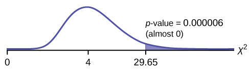
Probability statement:p-value = P(χ2 > 29.65) = 0.000006
Compare α and the p-value:
- α = 0.01
- p-value = 0.000006
So, α > p-value.
Make a decision: Since α > p-value, reject Ho.
This means you reject the belief that the distribution for the far western states is the same as that of the American population as a whole.
Conclusion: At the 1% significance level, from the data, there is sufficient evidence to conclude that the “number of televisions” distribution for the far western United States is different from the “number of televisions” distribution for the American population as a whole.
Press STAT and ENTER. Make sure to clear lists L1, L2, and L3 if they have data in them (see the note at the end of (Figure)). Into L1, put the observed frequencies 66, 119, 349, 60, 15. Into L2, put the expected frequencies .10*600, .16*600, .55*600, .11*600, .08*600. Arrow over to list L3 and up to the name area "L3". Enter (L1-L2)^2/L2 and ENTER. Press 2nd QUIT. Press 2nd LIST and arrow over to MATH. Press 5. You should see "sum" (Enter L3). Rounded to 2 decimal places, you should see 29.65. Press 2nd DISTR. Press 7 or Arrow down to 7:χ2cdf and press ENTER. Enter (29.65,1E99,4). Rounded to four places, you should see 5.77E-6 = .000006 (rounded to six decimal places), which is the p-value.
The newer TI-84 calculators have in STAT TESTS the test Chi2 GOF. To run the test, put the observed values (the data) into a first list and the expected values (the values you expect if the null hypothesis is true) into a second list. Press STAT TESTS and Chi2 GOF. Enter the list names for the Observed list and the Expected list. Enter the degrees of freedom and press calculate or draw. Make sure you clear any lists before you start.
The expected percentage of the number of pets students have in their homes is distributed (this is the given distribution for the student population of the United States) as in (Figure).
| Number of Pets | Percent |
|---|---|
| 0 | 18 |
| 1 | 25 |
| 2 | 30 |
| 3 | 18 |
| 4+ | 9 |
A random sample of 1,000 students from the Eastern United States resulted in the data in (Figure).
| Number of Pets | Frequency |
|---|---|
| 0 | 210 |
| 1 | 240 |
| 2 | 320 |
| 3 | 140 |
| 4+ | 90 |
At the 1% significance level, does it appear that the distribution “number of pets” of students in the Eastern United States is different from the distribution for the United States student population as a whole? What is the p-value?
Suppose you flip two coins 100 times. The results are 20 HH, 27 HT, 30 TH, and 23 TT. Are the coins fair? Test at a 5% significance level.
This problem can be set up as a goodness-of-fit problem. The sample space for flipping two fair coins is {HH, HT, TH, TT}. Out of 100 flips, you would expect 25 HH, 25 HT, 25 TH, and 25 TT. This is the expected distribution. The question, “Are the coins fair?” is the same as saying, “Does the distribution of the coins (20 HH, 27 HT, 30 TH, 23 TT) fit the expected distribution?”
Random Variable: Let X = the number of heads in one flip of the two coins. X takes on the values 0, 1, 2. (There are 0, 1, or 2 heads in the flip of two coins.) Therefore, the number of cells is three. Since X = the number of heads, the observed frequencies are 20 (for two heads), 57 (for one head), and 23 (for zero heads or both tails). The expected frequencies are 25 (for two heads), 50 (for one head), and 25 (for zero heads or both tails). This test is right-tailed.
H0: The coins are fair.
Ha: The coins are not fair.
Distribution for the test: where df = 3 – 1 = 2.
Calculate the test statistic:χ2 = 2.14
Graph:
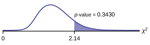
Probability statement:p-value = P(χ2 > 2.14) = 0.3430
Compare α and the p-value:
- α = 0.05
- p-value = 0.3430
α < p-value.
Make a decision: Since α < p-value, do not reject H0.
Conclusion: There is insufficient evidence to conclude that the coins are not fair.
Press STAT and ENTER. Make sure you clear lists L1, L2, and L3 if they have data in them. Into L1, put the observed frequencies 20, 57, 23. Into L2, put the expected frequencies 25, 50, 25. Arrow over to list L3 and up to the name area "L3". Enter (L1-L2)^2/L2 and ENTER. Press 2nd QUIT. Press 2nd LIST and arrow over to MATH. Press 5. You should see "sum".Enter L3. Rounded to two decimal places, you should see 2.14. Press 2nd DISTR. Arrow down to 7:χ2cdf (or press 7). Press ENTER. Enter 2.14,1E99,2). Rounded to four places, you should see .3430, which is the p-value.
The newer TI-84 calculators have in STAT TESTS the test Chi2 GOF. To run the test, put the observed values (the data) into a first list and the expected values (the values you expect if the null hypothesis is true) into a second list. Press STAT TESTS and Chi2 GOF. Enter the list names for the Observed list and the Expected list. Enter the degrees of freedom and press calculate or draw. Make sure you clear any lists before you start.
Students in a social studies class hypothesize that the literacy rates across the world for every region are 82%. (Figure) shows the actual literacy rates across the world broken down by region. What are the test statistic and the degrees of freedom?
| MDG Region | Adult Literacy Rate (%) |
|---|---|
| Developed Regions | 99.0 |
| Commonwealth of Independent States | 99.5 |
| Northern Africa | 67.3 |
| Sub-Saharan Africa | 62.5 |
| Latin America and the Caribbean | 91.0 |
| Eastern Asia | 93.8 |
| Southern Asia | 61.9 |
| South-Eastern Asia | 91.9 |
| Western Asia | 84.5 |
| Oceania | 66.4 |
References
Data from the U.S. Census Bureau
Data from the College Board. Available online at http://www.collegeboard.com.
Data from the U.S. Census Bureau, Current Population Reports.
Ma, Y., E.R. Bertone, E.J. Stanek III, G.W. Reed, J.R. Hebert, N.L. Cohen, P.A. Merriam, I.S. Ockene, “Association between Eating Patterns and Obesity in a Free-living US Adult Population.” American Journal of Epidemiology volume 158, no. 1, pages 85-92.
Ogden, Cynthia L., Margaret D. Carroll, Brian K. Kit, Katherine M. Flegal, “Prevalence of Obesity in the United States, 2009–2010.” NCHS Data Brief no. 82, January 2012. Available online at http://www.cdc.gov/nchs/data/databriefs/db82.pdf (accessed May 24, 2013).
Stevens, Barbara J., “Multi-family and Commercial Solid Waste and Recycling Survey.” Arlington Count, VA. Available online at http://www.arlingtonva.us/departments/EnvironmentalServices/SW/file84429.pdf (accessed May 24,2013).
Chapter Review
To assess whether a data set fits a specific distribution, you can apply the goodness-of-fit hypothesis test that uses the chi-square distribution. The null hypothesis for this test states that the data come from the assumed distribution. The test compares observed values against the values you would expect to have if your data followed the assumed distribution. The test is almost always right-tailed. Each observation or cell category must have an expected value of at least five.
Formula Review
 goodness-of-fit test statistic where:
O: observed values
E: expected values
k: number of different data cells or categories
df = k − 1 degrees of freedom
Determine the appropriate test to be used in the next three exercises.
An archeologist is calculating the distribution of the frequency of the number of artifacts she finds in a dig site. Based on previous digs, the archeologist creates an expected distribution broken down by grid sections in the dig site. Once the site has been fully excavated, she compares the actual number of artifacts found in each grid section to see if her expectation was accurate.
An economist is deriving a model to predict outcomes on the stock market. He creates a list of expected points on the stock market index for the next two weeks. At the close of each day’s trading, he records the actual points on the index. He wants to see how well his model matched what actually happened.
a goodness-of-fit test
A personal trainer is putting together a weight-lifting program for her clients. For a 90-day program, she expects each client to lift a specific maximum weight each week. As she goes along, she records the actual maximum weights her clients lifted. She wants to know how well her expectations met with what was observed.
Use the following information to answer the next five exercises: A teacher predicts that the distribution of grades on the final exam will be and they are recorded in (Figure).
| Grade | Proportion |
|---|---|
| A | 0.25 |
| B | 0.30 |
| C | 0.35 |
| D | 0.10 |
The actual distribution for a class of 20 is in (Figure).
| Grade | Frequency |
|---|---|
| A | 7 |
| B | 7 |
| C | 5 |
| D | 1 |
 ______
3
State the null and alternative hypotheses.
χ2 test statistic = ______
2.04
p-value = ______
At the 5% significance level, what can you conclude?
We decline to reject the null hypothesis. There is not enough evidence to suggest that the observed test scores are significantly different from the expected test scores.
Use the following information to answer the next nine exercises: The following data are real. The cumulative number of AIDS cases reported for Santa Clara County is broken down by ethnicity as in (Figure).
| Ethnicity | Number of Cases |
|---|---|
| White | 2,229 |
| Hispanic | 1,157 |
| Black/African-American | 457 |
| Asian, Pacific Islander | 232 |
| Total = 4,075 |
The percentage of each ethnic group in Santa Clara County is as in (Figure).
| Ethnicity | Percentage of total county population | Number expected (round to two decimal places) |
|---|---|---|
| White | 42.9% | 1748.18 |
| Hispanic | 26.7% | |
| Black/African-American | 2.6% | |
| Asian, Pacific Islander | 27.8% | |
| Total = 100% |
If the ethnicities of AIDS victims followed the ethnicities of the total county population, fill in the expected number of cases per ethnic group.
Perform a goodness-of-fit test to determine whether the occurrence of AIDS cases follows the ethnicities of the general population of Santa Clara County.
H0: _______
H0: the distribution of AIDS cases follows the ethnicities of the general population of Santa Clara County.
Ha: _______
Is this a right-tailed, left-tailed, or two-tailed test?
right-tailed
degrees of freedom = _______
χ2 test statistic = _______
2016.136
p-value = _______
Graph the situation. Label and scale the horizontal axis. Mark the mean and test statistic. Shade in the region corresponding to the p-value.
Let α = 0.05
Decision: ________________
Reason for the Decision: ________________
Conclusion (write out in complete sentences): ________________
Graph: Check student’s solution.
Decision: Reject the null hypothesis.
Reason for the Decision: p-value < alpha
Conclusion (write out in complete sentences): The make-up of AIDS cases does not fit the ethnicities of the general population of Santa Clara County.
Does it appear that the pattern of AIDS cases in Santa Clara County corresponds to the distribution of ethnic groups in this county? Why or why not?
Homework
For each problem, use a solution sheet to solve the hypothesis test problem. Go to (Figure) for the chi-square solution sheet. Round expected frequency to two decimal places.
1) A six-sided die is rolled 120 times. Fill in the expected frequency column. Then, conduct a hypothesis test to determine if the die is fair. The data in (Figure) are the result of the 120 rolls.
| Face Value | Frequency | Expected Frequency |
|---|---|---|
| 1 | 15 | |
| 2 | 29 | |
| 3 | 16 | |
| 4 | 15 | |
| 5 | 30 | |
| 6 | 15 |
2) The marital status distribution of the U.S. male population, ages 15 and older, is as shown in (Figure).
| Marital Status | Percent | Expected Frequency |
|---|---|---|
| never married | 31.3 | |
| married | 56.1 | |
| widowed | 2.5 | |
| divorced/separated | 10.1 |
3) Suppose that a random sample of 400 U.S. young adult males, 18 to 24 years old, yielded the following frequency distribution. We are interested in whether this age group of males fits the distribution of the U.S. adult population. Calculate the frequency one would expect when surveying 400 people. Fill in (Figure), rounding to two decimal places.
| Marital Status | Frequency |
|---|---|
| never married | 140 |
| married | 238 |
| widowed | 2 |
| divorced/separated | 20 |
| Marital Status | Percent | Expected Frequency |
|---|---|---|
| never married | 31.3 | 125.2 |
| married | 56.1 | 224.4 |
| widowed | 2.5 | 10 |
| divorced/separated | 10.1 | 40.4 |
Use the following information to answer the next two exercises:
The columns in (Figure) contain the Race/Ethnicity of U.S. Public Schools for a recent year, the percentages for the Advanced Placement Examinee Population for that class, and the Overall Student Population. Suppose the right column contains the result of a survey of 1,000 local students from that year who took an AP Exam.
| Race/Ethnicity | AP Examinee Population | Overall Student Population | Survey Frequency |
|---|---|---|---|
| Asian, Asian American, or Pacific Islander | 10.2% | 5.4% | 113 |
| Black or African-American | 8.2% | 14.5% | 94 |
| Hispanic or Latino | 15.5% | 15.9% | 136 |
| American Indian or Alaska Native | 0.6% | 1.2% | 10 |
| White | 59.4% | 61.6% | 604 |
| Not reported/other | 6.1% | 1.4% | 43 |
4) Perform a goodness-of-fit test to determine whether the local results follow the distribution of the U.S. overall student population based on ethnicity.
5) Perform a goodness-of-fit test to determine whether the local results follow the distribution of U.S. AP examinee population, based on ethnicity.
6) The City of South Lake Tahoe, CA, has an Asian population of 1,419 people, out of a total population of 23,609. Suppose that a survey of 1,419 self-reported Asians in the Manhattan, NY, area yielded the data in (Figure). Conduct a goodness-of-fit test to determine if the self-reported sub-groups of Asians in the Manhattan area fit that of the Lake Tahoe area.
| Race | Lake Tahoe Frequency | Manhattan Frequency |
|---|---|---|
| Asian Indian | 131 | 174 |
| Chinese | 118 | 557 |
| Filipino | 1,045 | 518 |
| Japanese | 80 | 54 |
| Korean | 12 | 29 |
| Vietnamese | 9 | 21 |
| Other | 24 | 66 |
Use the following information to answer the next two exercises:
UCLA conducted a survey of more than 263,000 college freshmen from 385 colleges in fall 2005. The results of students’ expected majors by gender were reported in The Chronicle of Higher Education (2/2/2006). Suppose a survey of 5,000 graduating females and 5,000 graduating males was done as a follow-up last year to determine what their actual majors were. The results are shown in the tables for (Figure) and (Figure). The second column in each table does not add to 100% because of rounding.
7) Conduct a goodness-of-fit test to determine if the actual college majors of graduating females fit the distribution of their expected majors.
| Major | Women – Expected Major | Women – Actual Major |
|---|---|---|
| Arts & Humanities | 14.0% | 670 |
| Biological Sciences | 8.4% | 410 |
| Business | 13.1% | 685 |
| Education | 13.0% | 650 |
| Engineering | 2.6% | 145 |
| Physical Sciences | 2.6% | 125 |
| Professional | 18.9% | 975 |
| Social Sciences | 13.0% | 605 |
| Technical | 0.4% | 15 |
| Other | 5.8% | 300 |
| Undecided | 8.0% | 420 |
8) Conduct a goodness-of-fit test to determine if the actual college majors of graduating males fit the distribution of their expected majors.
| Major | Men – Expected Major | Men – Actual Major |
|---|---|---|
| Arts & Humanities | 11.0% | 600 |
| Biological Sciences | 6.7% | 330 |
| Business | 22.7% | 1130 |
| Education | 5.8% | 305 |
| Engineering | 15.6% | 800 |
| Physical Sciences | 3.6% | 175 |
| Professional | 9.3% | 460 |
| Social Sciences | 7.6% | 370 |
| Technical | 1.8% | 90 |
| Other | 8.2% | 400 |
| Undecided | 6.6% | 340 |
Read the statement and decide whether it is true or false.
9) In a goodness-of-fit test, the expected values are the values we would expect if the null hypothesis were true.
10) In general, if the observed values and expected values of a goodness-of-fit test are not close together, then the test statistic can get very large and on a graph will be way out in the right tail.
11) Use a goodness-of-fit test to determine if high school principals believe that students are absent equally during the week or not.
12) The test to use to determine if a six-sided die is fair is a goodness-of-fit test.
13) In a goodness-of fit test, if the p-value is 0.0113, in general, do not reject the null hypothesis.
14) A sample of 212 commercial businesses was surveyed for recycling one commodity; a commodity here means any one type of recyclable material such as plastic or aluminum. (Figure) shows the business categories in the survey, the sample size of each category, and the number of businesses in each category that recycle one commodity. Based on the study, on average half of the businesses were expected to be recycling one commodity. As a result, the last column shows the expected number of businesses in each category that recycle one commodity. At the 5% significance level, perform a hypothesis test to determine if the observed number of businesses that recycle one commodity follows the uniform distribution of the expected values.
| Business Type | Number in class | Observed Number that recycle one commodity | Expected number that recycle one commodity |
|---|---|---|---|
| Office | 35 | 19 | 17.5 |
| Retail/Wholesale | 48 | 27 | 24 |
| Food/Restaurants | 53 | 35 | 26.5 |
| Manufacturing/Medical | 52 | 21 | 26 |
| Hotel/Mixed | 24 | 9 | 12 |
15) (Figure) contains information from a survey among 499 participants classified according to their age groups. The second column shows the percentage of obese people per age class among the study participants. The last column comes from a different study at the national level that shows the corresponding percentages of obese people in the same age classes in the USA. Perform a hypothesis test at the 5% significance level to determine whether the survey participants are a representative sample of the USA obese population.
| Age Class (Years) | Obese Expected (Percentage) | Obese-Observed (Frequencies) |
|---|---|---|
| 20–30 | 22.4 | 122 |
| 31–40 | 18.6 | 104 |
| 41–50 | 12.8 | 78 |
| 51–60 | 10.4 | 64 |
| 61–70 | 35.8 | 168 |
Answers to odd questions
3)
- The data fits the distribution.
- The data does not fit the distribution.
- 3
- chi-square distribution with df = 3
- 19.27
- 0.0002
- Check student’s solution.
-
- Alpha = 0.05
- Decision: Reject null
- Reason for decision: p-value < alpha
- Conclusion: Data does not fit the distribution.
5)
- H0: The local results follow the distribution of the U.S. AP examinee population
- Ha: The local results do not follow the distribution of the U.S. AP examinee population
- df = 5
- chi-square distribution with df = 5
- chi-square test statistic = 13.4
- p-value = 0.0199
- Check student’s solution.
-
- Alpha = 0.05
- Decision: Reject null when a = 0.05
- Reason for Decision: p-value < alpha
- Conclusion: Local data do not fit the AP Examinee Distribution.
- Decision: Do not reject null when a = 0.01
- Conclusion: There is insufficient evidence to conclude that local data do not follow the distribution of the U.S. AP examinee distribution.
7)
- H0: The actual college majors of graduating females fit the distribution of their expected majors
- Ha: The actual college majors of graduating females do not fit the distribution of their expected majors
- df = 10
- chi-square distribution with df = 10
- test statistic = 11.48
- p-value = 0.3211
- Check student’s solution.
-
- Alpha = 0.05
- Decision: Do not reject null when a = 0.05 and a = 0.01
- Reason for decision: p-value > alpha
- Conclusion: There is insufficient evidence to conclude that the distribution of actual college majors of graduating females do not fit the distribution of their expected majors.
9) true
11) true
13) false
15)
- H0: Surveyed obese fit the distribution of expected obese
- Ha: Surveyed obese do not fit the distribution of expected obese
- df = 4
- chi-square distribution with df = 4
- test statistic = 507.6
- p-value = 0
- Check student’s solution.
-
- Alpha: 0.05
- Decision: Reject the null hypothesis.
- Reason for decision: p-value < alpha
- Conclusion: At the 5% level of significance, from the data, there is sufficient evidence to conclude that the surveyed obese do not fit the distribution of expected obese.
