Chapter 13.4: Facts About the F Distribution
Here are some facts about the F distribution.
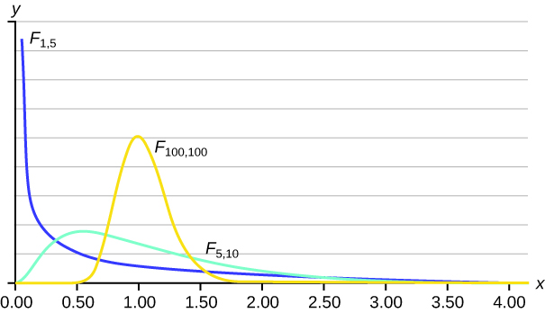
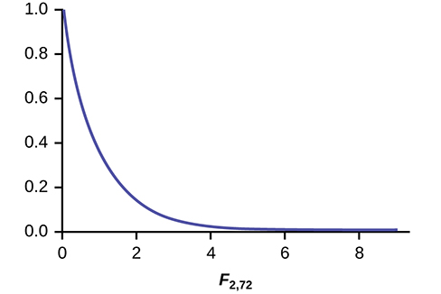
- The curve is not symmetrical but skewed to the right.
- There is a different curve for each set of dfs.
- The F statistic is greater than or equal to zero.
- As the degrees of freedom for the numerator and for the denominator get larger, the curve approximates the normal.
- Other uses for the F distribution include comparing two variances and two-way Analysis of Variance. Two-Way Analysis is beyond the scope of this chapter.
Let’s return to the slicing tomato exercise in (Figure). The means of the tomato yields under the five mulching conditions are represented by μ1, μ2, μ3, μ4, μ5. We will conduct a hypothesis test to determine if all means are the same or at least one is different. Using a significance level of 5%, test the null hypothesis that there is no difference in mean yields among the five groups against the alternative hypothesis that at least one mean is different from the rest.
The null and alternative hypotheses are:
H0: μ1 = μ2 = μ3 = μ4 = μ5
Ha: μi ≠ μj some i ≠ j
The one-way ANOVA results are shown in (Figure)
| Source of Variation | Sum of Squares (SS) | Degrees of Freedom (df) | Mean Square (MS) | F |
|---|---|---|---|---|
| Factor (Between) | 36,648,561 | 5 – 1 = 4 |  |
 |
| Error (Within) | 20,446,726 | 15 – 5 = 10 |  |
|
| Total | 57,095,287 | 15 – 1 = 14 |
Distribution for the test: F4,10
df(num) = 5 – 1 = 4
df(denom) = 15 – 5 = 10
Test statistic:F = 4.4810
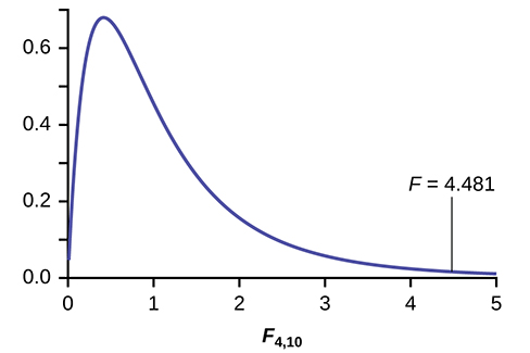
Probability Statement:p-value = P(F > 4.481) = 0.0248.
Compare α and the p-value:α = 0.05, p-value = 0.0248
Make a decision: Since α > p-value, we reject H0.
Conclusion: At the 5% significance level, we have reasonably strong evidence that differences in mean yields for slicing tomato plants grown under different mulching conditions are unlikely to be due to chance alone. We may conclude that at least some of mulches led to different mean yields.
To find these results on the calculator:
Press STAT. Press 1:EDIT. Put the data into the lists L1, L2, L3, L4, L5.
Press STAT, and arrow over to TESTS, and arrow down to ANOVA. Press ENTER, and then enter L1, L2, L3, L4, L5). Press ENTER. You will see that the values in the foregoing ANOVA table are easily produced by the calculator, including the test statistic and the p-value of the test.
The calculator displays:
F = 4.4810
p = 0.0248 (p-value)
Factor
df = 4
SS = 36648560.9
MS = 9162140.23
Error
df = 10
SS = 20446726
MS = 2044672.6
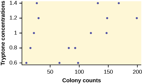
MRSA, or Staphylococcus aureus, can cause a serious bacterial infections in hospital patients. (Figure) shows various colony counts from different patients who may or may not have MRSA. The data from the table is plotted in Figure 13.5.
| Conc = 0.6 | Conc = 0.8 | Conc = 1.0 | Conc = 1.2 | Conc = 1.4 |
|---|---|---|---|---|
| 9 | 16 | 22 | 30 | 27 |
| 66 | 93 | 147 | 199 | 168 |
| 98 | 82 | 120 | 148 | 132 |
Plot of the data for the different concentrations:
Test whether the mean number of colonies are the same or are different. Construct the ANOVA table (by hand or by using a TI-83, 83+, or 84+ calculator), find the p-value, and state your conclusion. Use a 5% significance level.
Four sororities took a random sample of sisters regarding their grade means for the past term. The results are shown in (Figure).
| Sorority 1 | Sorority 2 | Sorority 3 | Sorority 4 |
|---|---|---|---|
| 2.17 | 2.63 | 2.63 | 3.79 |
| 1.85 | 1.77 | 3.78 | 3.45 |
| 2.83 | 3.25 | 4.00 | 3.08 |
| 1.69 | 1.86 | 2.55 | 2.26 |
| 3.33 | 2.21 | 2.45 | 3.18 |
Using a significance level of 1%, is there a difference in mean grades among the sororities?
Let μ1, μ2, μ3, μ4 be the population means of the sororities. Remember that the null hypothesis claims that the sorority groups are from the same normal distribution. The alternate hypothesis says that at least two of the sorority groups come from populations with different normal distributions. Notice that the four sample sizes are each five.
This is an example of a balanced design, because each factor (i.e., sorority) has the same number of observations.
H0: μ1 = μ2 = μ3 = μ4
Ha: Not all of the means μ1, μ2, μ3, μ4 are equal.
Distribution for the test:F3,16
where k = 4 groups and n = 20 samples in total
df(num)= k – 1 = 4 – 1 = 3
df(denom) = n – k = 20 – 4 = 16
Calculate the test statistic:F = 2.23
Graph:
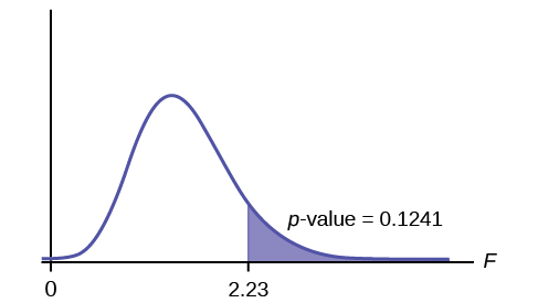
Probability statement:p-value = P(F > 2.23) = 0.1241
Compare α and the p-value:α = 0.01
p-value = 0.1241
α < p-value
Make a decision: Since α < p-value, you cannot reject H0.
Conclusion: There is not sufficient evidence to conclude that there is a difference among the mean grades for the sororities.
Put the data into lists L1, L2, L3, and L4. Press STAT and arrow over to TESTS. Arrow down to F:ANOVA. Press ENTER and Enter (L1,L2,L3,L4).
The calculator displays the F statistic, the p-value and the values for the one-way ANOVA table:
F = 2.2303
p = 0.1241 (p-value)
Factor
df = 3
SS = 2.88732
MS = 0.96244
Error
df = 16
SS = 6.9044
MS = 0.431525
Four sports teams took a random sample of players regarding their GPAs for the last year. The results are shown in (Figure).
| Basketball | Baseball | Hockey | Lacrosse |
|---|---|---|---|
| 3.6 | 2.1 | 4.0 | 2.0 |
| 2.9 | 2.6 | 2.0 | 3.6 |
| 2.5 | 3.9 | 2.6 | 3.9 |
| 3.3 | 3.1 | 3.2 | 2.7 |
| 3.8 | 3.4 | 3.2 | 2.5 |
Use a significance level of 5%, and determine if there is a difference in GPA among the teams.
A fourth grade class is studying the environment. One of the assignments is to grow bean plants in different soils. Tommy chose to grow his bean plants in soil found outside his classroom mixed with dryer lint. Tara chose to grow her bean plants in potting soil bought at the local nursery. Nick chose to grow his bean plants in soil from his mother’s garden. No chemicals were used on the plants, only water. They were grown inside the classroom next to a large window. Each child grew five plants. At the end of the growing period, each plant was measured, producing the data (in inches) in (Figure).
| Tommy’s Plants | Tara’s Plants | Nick’s Plants |
|---|---|---|
| 24 | 25 | 23 |
| 21 | 31 | 27 |
| 23 | 23 | 22 |
| 30 | 20 | 30 |
| 23 | 28 | 20 |
Does it appear that the three media in which the bean plants were grown produce the same mean height? Test at a 3% level of significance.
This time, we will perform the calculations that lead to the F’ statistic. Notice that each group has the same number of plants, so we will use the formula F’ =  .
.
First, calculate the sample mean and sample variance of each group.
| Tommy’s Plants | Tara’s Plants | Nick’s Plants | |
|---|---|---|---|
| Sample Mean | 24.2 | 25.4 | 24.4 |
| Sample Variance | 11.7 | 18.3 | 16.3 |
Next, calculate the variance of the three group means (Calculate the variance of 24.2, 25.4, and 24.4). Variance of the group means = 0.413 = 
Then MSbetween =  = (5)(0.413) where n = 5 is the sample size (number of plants each child grew).
Calculate the mean of the three sample variances (Calculate the mean of 11.7, 18.3, and 16.3). Mean of the sample variances = 15.433 = s2pooled
Then MSwithin = s2pooled = 15.433.
The F statistic (or F ratio) is 
The dfs for the numerator = the number of groups – 1 = 3 – 1 = 2.
The dfs for the denominator = the total number of samples – the number of groups = 15 – 3 = 12
The distribution for the test is F2,12 and the F statistic is F = 0.134
The p-value is P(F > 0.134) = 0.8759.
Decision: Since α = 0.03 and the p-value = 0.8759, do not reject H0. (Why?)
Conclusion: With a 3% level of significance, from the sample data, the evidence is not sufficient to conclude that the mean heights of the bean plants are different.
To calculate the p-value:
*Press 2nd DISTR
*Arrow down to Fcdf(and press ENTER.
*Enter 0.134, E99, 2, 12)
*Press ENTER
The p-value is 0.8759.
Another fourth grader also grew bean plants, but this time in a jelly-like mass. The heights were (in inches) 24, 28, 25, 30, and 32. Do a one-way ANOVA test on the four groups. Are the heights of the bean plants different? Use the same method as shown in (Figure).
From the class, create four groups of the same size as follows: men under 22, men at least 22, women under 22, women at least 22. Have each member of each group record the number of states in the United States he or she has visited. Run an ANOVA test to determine if the average number of states visited in the four groups are the same. Test at a 1% level of significance. Use one of the solution sheets in (Figure).
References
Data from a fourth grade classroom in 1994 in a private K – 12 school in San Jose, CA.
Hand, D.J., F. Daly, A.D. Lunn, K.J. McConway, and E. Ostrowski. A Handbook of Small Datasets: Data for Fruitfly Fecundity. London: Chapman & Hall, 1994.
Hand, D.J., F. Daly, A.D. Lunn, K.J. McConway, and E. Ostrowski. A Handbook of Small Datasets. London: Chapman & Hall, 1994, pg. 50.
Hand, D.J., F. Daly, A.D. Lunn, K.J. McConway, and E. Ostrowski. A Handbook of Small Datasets. London: Chapman & Hall, 1994, pg. 118.
“MLB Standings – 2012.” Available online at http://espn.go.com/mlb/standings/_/year/2012.
Mackowiak, P. A., Wasserman, S. S., and Levine, M. M. (1992), “A Critical Appraisal of 98.6 Degrees F, the Upper Limit of the Normal Body Temperature, and Other Legacies of Carl Reinhold August Wunderlich,” Journal of the American Medical Association, 268, 1578-1580.
Chapter Review
The graph of the F distribution is always positive and skewed right, though the shape can be mounded or exponential depending on the combination of numerator and denominator degrees of freedom. The F statistic is the ratio of a measure of the variation in the group means to a similar measure of the variation within the groups. If the null hypothesis is correct, then the numerator should be small compared to the denominator. A small F statistic will result, and the area under the F curve to the right will be large, representing a large p-value. When the null hypothesis of equal group means is incorrect, then the numerator should be large compared to the denominator, giving a large F statistic and a small area (small p-value) to the right of the statistic under the F curve.
When the data have unequal group sizes (unbalanced data), then techniques from (Figure) need to be used for hand calculations. In the case of balanced data (the groups are the same size) however, simplified calculations based on group means and variances may be used. In practice, of course, software is usually employed in the analysis. As in any analysis, graphs of various sorts should be used in conjunction with numerical techniques. Always look of your data!
An F statistic can have what values?
What happens to the curves as the degrees of freedom for the numerator and the denominator get larger?
The curves approximate the normal distribution.
Use the following information to answer the next seven exercise. Four basketball teams took a random sample of players regarding how high each player can jump (in inches). The results are shown in (Figure).
| Team 1 | Team 2 | Team 3 | Team 4 | Team 5 |
|---|---|---|---|---|
| 36 | 32 | 48 | 38 | 41 |
| 42 | 35 | 50 | 44 | 39 |
| 51 | 38 | 39 | 46 | 40 |
What is the df(num)?
What is the df(denom)?
ten
What are the Sum of Squares and Mean Squares Factors?
What are the Sum of Squares and Mean Squares Errors?
SS = 237.33; MS = 23.73
What is the F statistic?
What is the p-value?
0.1614
At the 5% significance level, is there a difference in the mean jump heights among the teams?
Use the following information to answer the next seven exercises. A video game developer is testing a new game on three different groups. Each group represents a different target market for the game. The developer collects scores from a random sample from each group. The results are shown in (Figure)
| Group A | Group B | Group C |
|---|---|---|
| 101 | 151 | 101 |
| 108 | 149 | 109 |
| 98 | 160 | 198 |
| 107 | 112 | 186 |
| 111 | 126 | 160 |
What is the df(num)?
two
What is the df(denom)?
What are the SSbetween and MSbetween?
SS = 5,700.4;
MS = 2,850.2
What are the SSwithin and MSwithin?
What is the F Statistic?
3.6101
What is the p-value?
At the 10% significance level, are the scores among the different groups different?
Yes, there is enough evidence to show that the scores among the groups are statistically significant at the 10% level.
Use the following information to answer the next three exercises. Suppose a group is interested in determining whether teenagers obtain their drivers licenses at approximately the same average age across the country. Suppose that the following data are randomly collected from five teenagers in each region of the country. The numbers represent the age at which teenagers obtained their drivers licenses.
| Northeast | South | West | Central | East | |
|---|---|---|---|---|---|
| 16.3 | 16.9 | 16.4 | 16.2 | 17.1 | |
| 16.1 | 16.5 | 16.5 | 16.6 | 17.2 | |
| 16.4 | 16.4 | 16.6 | 16.5 | 16.6 | |
| 16.5 | 16.2 | 16.1 | 16.4 | 16.8 | |
 |
________ | ________ | ________ | ________ | ________ |
 |
________ | ________ | ________ | ________ | ________ |
Enter the data into your calculator or computer.
p-value = ______
State the decisions and conclusions (in complete sentences) for the following preconceived levels of α.
α = 0.05
a. Decision: ____________________________
b. Conclusion: ____________________________
α = 0.01
a. Decision: ____________________________
b. Conclusion: ____________________________
Homework
Use a solution sheet to conduct the following hypothesis tests. The solution sheet can be found in (Figure).
1) Three students, Linda, Tuan, and Javier, are given five laboratory rats each for a nutritional experiment. Each rat’s weight is recorded in grams. Linda feeds her rats Formula A, Tuan feeds his rats Formula B, and Javier feeds his rats Formula C. At the end of a specified time period, each rat is weighed again, and the net gain in grams is recorded. Using a significance level of 10%, test the hypothesis that the three formulas produce the same mean weight gain.
| Linda’s rats | Tuan’s rats | Javier’s rats |
|---|---|---|
| 43.5 | 47.0 | 51.2 |
| 39.4 | 40.5 | 40.9 |
| 41.3 | 38.9 | 37.9 |
| 46.0 | 46.3 | 45.0 |
| 38.2 | 44.2 | 48.6 |
2) A grassroots group opposed to a proposed increase in the gas tax claimed that the increase would hurt working-class people the most, since they commute the farthest to work. Suppose that the group randomly surveyed 24 individuals and asked them their daily one-way commuting mileage. The results are in (Figure). Using a 5% significance level, test the hypothesis that the three mean commuting mileages are the same.
| working-class | professional (middle incomes) | professional (wealthy) |
|---|---|---|
| 17.8 | 16.5 | 8.5 |
| 26.7 | 17.4 | 6.3 |
| 49.4 | 22.0 | 4.6 |
| 9.4 | 7.4 | 12.6 |
| 65.4 | 9.4 | 11.0 |
| 47.1 | 2.1 | 28.6 |
| 19.5 | 6.4 | 15.4 |
| 51.2 | 13.9 | 9.3 |
Use the following information to answer the next two exercises.(Figure) lists the number of pages in four different types of magazines.
| home decorating | news | health | computer |
|---|---|---|---|
| 172 | 87 | 82 | 104 |
| 286 | 94 | 153 | 136 |
| 163 | 123 | 87 | 98 |
| 205 | 106 | 103 | 207 |
| 197 | 101 | 96 | 146 |
Using a significance level of 5%, test the hypothesis that the four magazine types have the same mean length.
3) Eliminate one magazine type that you now feel has a mean length different from the others. Redo the hypothesis test, testing that the remaining three means are statistically the same. Use a new solution sheet. Based on this test, are the mean lengths for the remaining three magazines statistically the same?
4) A researcher wants to know if the mean times (in minutes) that people watch their favorite news station are the same. Suppose that (Figure) shows the results of a study.
| CNN | FOX | Local |
|---|---|---|
| 45 | 15 | 72 |
| 12 | 43 | 37 |
| 18 | 68 | 56 |
| 38 | 50 | 60 |
| 23 | 31 | 51 |
| 35 | 22 |
Assume that all distributions are normal, the four population standard deviations are approximately the same, and the data were collected independently and randomly. Use a level of significance of 0.05.
5) Are the means for the final exams the same for all statistics class delivery types? (Figure) shows the scores on final exams from several randomly selected classes that used the different delivery types.
| Online | Hybrid | Face-to-Face |
|---|---|---|
| 72 | 83 | 80 |
| 84 | 73 | 78 |
| 77 | 84 | 84 |
| 80 | 81 | 81 |
| 81 | 86 | |
| 79 | ||
| 82 |
Assume that all distributions are normal, the four population standard deviations are approximately the same, and the data were collected independently and randomly. Use a level of significance of 0.05.
6) Are the mean number of times a month a person eats out the same for whites, blacks, Hispanics and Asians? Suppose that (Figure) shows the results of a study.
| White | Black | Hispanic | Asian |
|---|---|---|---|
| 6 | 4 | 7 | 8 |
| 8 | 1 | 3 | 3 |
| 2 | 5 | 5 | 5 |
| 4 | 2 | 4 | 1 |
| 6 | 6 | 7 |
Assume that all distributions are normal, the four population standard deviations are approximately the same, and the data were collected independently and randomly. Use a level of significance of 0.05.
7) Are the mean numbers of daily visitors to a ski resort the same for the three types of snow conditions? Suppose that (Figure) shows the results of a study.
| Powder | Machine Made | Hard Packed |
|---|---|---|
| 1,210 | 2,107 | 2,846 |
| 1,080 | 1,149 | 1,638 |
| 1,537 | 862 | 2,019 |
| 941 | 1,870 | 1,178 |
| 1,528 | 2,233 | |
| 1,382 |
Assume that all distributions are normal, the four population standard deviations are approximately the same, and the data were collected independently and randomly. Use a level of significance of 0.05.
8) Sanjay made identical paper airplanes out of three different weights of paper, light, medium and heavy. He made four airplanes from each of the weights, and launched them himself across the room. Here are the distances (in meters) that his planes flew.
| Paper Type/Trial | Trial 1 | Trial 2 | Trial 3 | Trial 4 |
|---|---|---|---|---|
| Heavy | 5.1 meters | 3.1 meters | 4.7 meters | 5.3 meters |
| Medium | 4 meters | 3.5 meters | 4.5 meters | 6.1 meters |
| Light | 3.1 meters | 3.3 meters | 2.1 meters | 1.9 meters |
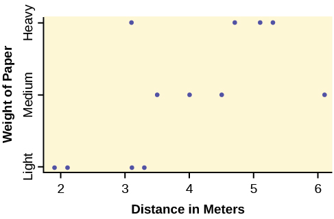
- Take a look at the data in the graph. Look at the spread of data for each group (light, medium, heavy). Does it seem reasonable to assume a normal distribution with the same variance for each group? Yes or No.
- Why is this a balanced design?
- Calculate the sample mean and sample standard deviation for each group.
- Does the weight of the paper have an effect on how far the plane will travel? Use a 1% level of significance. Complete the test using the method shown in the bean plant example in (Figure).
- variance of the group means __________
- MSbetween= ___________
- mean of the three sample variances ___________
- MSwithin = _____________
- F statistic = ____________
- df(num) = __________, df(denom) = ___________
- number of groups _______
- number of observations _______
- p-value = __________ (P(F > _______) = __________)
- Graph the p-value.
- decision: _______________________
- conclusion: _______________________________________________________________
9) DDT is a pesticide that has been banned from use in the United States and most other areas of the world. It is quite effective, but persisted in the environment and over time became seen as harmful to higher-level organisms. Famously, egg shells of eagles and other raptors were believed to be thinner and prone to breakage in the nest because of ingestion of DDT in the food chain of the birds.
An experiment was conducted on the number of eggs (fecundity) laid by female fruit flies. There are three groups of flies. One group was bred to be resistant to DDT (the RS group). Another was bred to be especially susceptible to DDT (SS). Finally there was a control line of non-selected or typical fruitflies (NS). Here are the data:
| RS | SS | NS | RS | SS | NS |
|---|---|---|---|---|---|
| 12.8 | 38.4 | 35.4 | 22.4 | 23.1 | 22.6 |
| 21.6 | 32.9 | 27.4 | 27.5 | 29.4 | 40.4 |
| 14.8 | 48.5 | 19.3 | 20.3 | 16 | 34.4 |
| 23.1 | 20.9 | 41.8 | 38.7 | 20.1 | 30.4 |
| 34.6 | 11.6 | 20.3 | 26.4 | 23.3 | 14.9 |
| 19.7 | 22.3 | 37.6 | 23.7 | 22.9 | 51.8 |
| 22.6 | 30.2 | 36.9 | 26.1 | 22.5 | 33.8 |
| 29.6 | 33.4 | 37.3 | 29.5 | 15.1 | 37.9 |
| 16.4 | 26.7 | 28.2 | 38.6 | 31 | 29.5 |
| 20.3 | 39 | 23.4 | 44.4 | 16.9 | 42.4 |
| 29.3 | 12.8 | 33.7 | 23.2 | 16.1 | 36.6 |
| 14.9 | 14.6 | 29.2 | 23.6 | 10.8 | 47.4 |
| 27.3 | 12.2 | 41.7 |
The values are the average number of eggs laid daily for each of 75 flies (25 in each group) over the first 14 days of their lives. Using a 1% level of significance, are the mean rates of egg selection for the three strains of fruitfly different? If so, in what way? Specifically, the researchers were interested in whether or not the selectively bred strains were different from the nonselected line, and whether the two selected lines were different from each other.
10) Calculate 95% confidence intervals for the mean body temperature in each group and comment about the confidence intervals.
| FL | FH | ML | MH | FL | FH | ML | MH |
|---|---|---|---|---|---|---|---|
| 96.4 | 96.8 | 96.3 | 96.9 | 98.4 | 98.6 | 98.1 | 98.6 |
| 96.7 | 97.7 | 96.7 | 97 | 98.7 | 98.6 | 98.1 | 98.6 |
| 97.2 | 97.8 | 97.1 | 97.1 | 98.7 | 98.6 | 98.2 | 98.7 |
| 97.2 | 97.9 | 97.2 | 97.1 | 98.7 | 98.7 | 98.2 | 98.8 |
| 97.4 | 98 | 97.3 | 97.4 | 98.7 | 98.7 | 98.2 | 98.8 |
| 97.6 | 98 | 97.4 | 97.5 | 98.8 | 98.8 | 98.2 | 98.8 |
| 97.7 | 98 | 97.4 | 97.6 | 98.8 | 98.8 | 98.3 | 98.9 |
| 97.8 | 98 | 97.4 | 97.7 | 98.8 | 98.8 | 98.4 | 99 |
| 97.8 | 98.1 | 97.5 | 97.8 | 98.8 | 98.9 | 98.4 | 99 |
| 97.9 | 98.3 | 97.6 | 97.9 | 99.2 | 99 | 98.5 | 99 |
| 97.9 | 98.3 | 97.6 | 98 | 99.3 | 99 | 98.5 | 99.2 |
| 98 | 98.3 | 97.8 | 98 | 99.1 | 98.6 | 99.5 | |
| 98.2 | 98.4 | 97.8 | 98 | 99.1 | 98.6 | ||
| 98.2 | 98.4 | 97.8 | 98.3 | 99.2 | 98.7 | ||
| 98.2 | 98.4 | 97.9 | 98.4 | 99.4 | 99.1 | ||
| 98.2 | 98.4 | 98 | 98.4 | 99.9 | 99.3 | ||
| 98.2 | 98.5 | 98 | 98.6 | 100 | 99.4 | ||
| 98.2 | 98.6 | 98 | 98.6 | 100.8 |
Answers to odd questions
1)
- H0: µL = µT = µJ
- Ha: at least any two of the means are different
- df(num) = 2; df(denom) = 12
- F distribution
- 0.67
- 0.5305
- Check student’s solution.
- Decision: Do not reject null hypothesis; Conclusion: There is insufficient evidence to conclude that the means are different.
3)
- Ha: µc = µn = µh
- At least any two of the magazines have different mean lengths.
- df(num) = 2, df(denom) = 12
- F distribtuion
- F = 15.28
- p-value = 0.0005
- Check student’s solution.
-
- Alpha: 0.05
- Decision: Reject the Null Hypothesis.
- Reason for decision: p-value < alpha
- Conclusion: There is sufficient evidence to conclude that the mean lengths of the magazines are different.
5)
- H0: μo = μh = μf
- At least two of the means are different.
- df(n) = 2, df(d) = 13
- F2,13
- 0.64
- 0.5437
- Check student’s solution.
-
- Alpha: 0.05
- Decision: Do not reject the null hypothesis.
- Reason for decision: p-value > alpha
- Conclusion: The mean scores of different class delivery are not different.
7)
- H0: μp = μm = μh
- At least any two of the means are different.
- df(n) = 2, df(d) = 12
- F2,12
- 3.13
- 0.0807
- Check student’s solution.
-
- Alpha: 0.05
- Decision: Do not reject the null hypothesis.
- Reason for decision: p-value > alpha
- Conclusion: There is not sufficient evidence to conclude that the mean numbers of daily visitors are different.
9)
Here is a chart of the three groups:
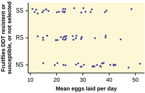
The data appear normally distributed from the chart and of similar spread. There do not appear to be any serious outliers, so we may proceed with our ANOVA calculations, to see if we have good evidence of a difference between the three groups.
H0: μ1 = μ2 = μ3;
Ha: μi ≠ μj some i ≠ j.
Define μ1, μ2, μ3, as the population mean number of eggs laid by the three groups of fruit flies.
F statistic = 8.6657;
p-value = 0.0004
Decision: Since the p-value is less than the level of significance of 0.01, we reject the null hypothesis.
Conclusion: We have good evidence that the average number of eggs laid during the first 14 days of life for these three strains of fruitflies are different.
Interestingly if you perform a two sample t-test to compare the RS and NS groups they are significantly different (p = 0.0013). Similarly, SS and NS are significantly different (p = 0.0006). However, the two selected groups, RS and SS are not significantly different (p = 0.5176). Thus we appear to have good evidence that selection either for resistance or for susceptibility involves a reduced rate of egg production (for these specific strains) as compared to flies that were not selected for resistance or susceptibility to DDT. Here, genetic selection has apparently involved a loss of fecundity.
The data shown is the recorded body temperatures of 130 subjects as estimated from available histograms.
Traditionally we are taught that the normal human body temperature is 98.6 F. This is not quite correct for everyone. Are the mean temperatures among the four groups different?
