Chapter 7 Wrap Up

Adapted by John Morgan Russell; from Barbara Illowsky and Susan Dean, David Diez, Mine Cetinkaya-Rundel and Christopher D. Barr; Julie Vu and David Harrington

Chapter 7 Wrap Up

Concept Check

Section Reviews

7.1 Sampling Distribution of the Sample Mean

In many cases, the researcher does not know the population standard deviation, σ, of the measure being studied. In these cases, it is common to use the sample standard deviation, s, as an estimate of σ. The normal distribution creates accurate confidence intervals when σ is known, but it is not as accurate when s is used as an estimate. In this case, the Student’s t-distribution is much better. Define a t-score using the following formula:

$t= \frac{\overline{x}- \mu }{s}{\sqrt{n}}}$

When using inference techniques for a single population mean the following distributions should be used under certain circumstances:

A Student’s t-test should be used if the data come from a simple, random sample and the population is approximately normally distributed, or the sample size is large, with an unknown standard deviation.
The normal (Z) test will work if the data come from a simple, random sample and the population is approximately normally distributed, or the sample size is large, with a known standard deviation.

We can construct confidence Interval with the corresponding critical value or perform Hypothesis tests with the correct Tests statistic

7.2 Inference for the Mean in Practice

The t-score follows the Student’s t-distribution with n – 1 degrees of freedom. The confidence interval under this distribution is calculated with EBM = $\left({t}_{\frac{\alpha }{2}}\right)\frac{s}{\sqrt{n}}$ where ${t}_{\frac{\alpha }{2}}$ is the t-score with area to the right equal to $\frac{\alpha }{2}$ , s is the sample standard deviation, and n is the sample size. Use a table, calculator, or computer to find ${t}_{\frac{\alpha }{2}}$ for a given α.

s = the standard deviation of sample values.

$t= \frac{\overline{x}-\mu }{\frac{s}{\sqrt{n}}}$ is the formula for the t-score which measures how far away a measure is from the population mean in the Student’s t-distribution

df = n – 1; the degrees of freedom for a Student’s t-distribution where n represents the size of the sample

T~t_df the random variable, T, has a Student’s t-distribution with df degrees of freedom

$EBM={t}_{\frac{\alpha }{2}}\frac{s}{\sqrt{n}}$ = the error bound for the population mean when the population standard deviation is unknown

${t}_{\frac{\alpha }{2}}$ is the t-score in the Student’s t-distribution with area to the right equal to $\frac{\alpha }{2}$

The general form for a confidence interval for a single mean, population standard deviation unknown, Student’s t is given by (lower bound, upper bound)
= (point estimate – EBM, point estimate + EBM)
= $\left(\overline{x}-\frac{ts}{\sqrt{n}},\overline{x}\text{+ }\frac{ts}{\sqrt{n}}\right)$

7.3 Sampling Distribution of the Sample Proportion

When testing a single population proportion use a normal test for a single population proportion if the data comes from a simple, random sample, fill the requirements for a binomial distribution, and the mean number of success and the mean number of failures satisfy the conditions: np > 5 and nq > n where n is the sample size, p is the probability of a success, and q is the probability of a failure.

Some statistical measures, like many survey questions, measure categorical rather than quantitative data. In this case, the population parameter being estimated is a proportion.

The variable p̂ = x / n, where x represents the number of successes and n represents the sample size, is the sample proportion and serves as the point estimate for the true population proportion.

The variable p̂ has a binomial distribution that can be approximated with the normal distribution shown below given you meet the criteria.

$\hat{p}\text{~N}\left(p,\sqrt{\frac{p(1-p}{n}}\right)$

7.4 Inference for a Proportion

It is possible to create a confidence interval for the true population proportion following procedures similar to those used in creating confidence intervals for population means. The formulas are slightly different, but they follow the same reasoning.

Let p̂ represent the sample proportion, x/n, where x represents the number of successes and n represents the sample size. Let q = 1 – p̂.

The general form of a CI is:

(lower bound, upper bound)

Then the confidence interval for a population proportion is given by the following formula:

$\left(\hat{p}-MoE,\hat{p}+MoE\right)$

The Margin of Error (MoE) for a proportion is:

${z}_{\frac{\alpha }{2}\sqrt{\frac{\hat{p}\hat{q}}{n}}$

Putting that together:

$\left(\hat{p}-z\sqrt{\frac{\hat{p}\hat{q}}{n}},\hat{p}+z\sqrt{\frac{\hat{p}\hat{q}}{n}}\right)$

7.5 Behavior of Confidence Intervals for a Proportion

A CI for p behaves similarly to what we have seen for Z CIs for µ as far as Confidence levels and sample sizes.

provides the number of participants needed to estimate the population proportion with confidence 1 – α and margin of error MoE.

$n=\left(\frac{{z}_{\frac{\alpha }{2}}}{MoE}\right)^{2}\text{p(1-p)}$

Options to plug in for p:

If you have prior information such as a previous sample and can calculate a point estimate $\left(\hat{p}\right)$ plug it in!
You can use your best guess at p
You can use a “conservative” estimate of p, 0.5.*

The “plus four” method for calculating confidence intervals is an attempt to balance the error introduced by using estimates of the population proportion when calculating the standard deviation of the sampling distribution. Use:

$\hat{p}=\frac{x+2}{n+4}$

Then find the confidence interval. When sample sizes are small, this method has been demonstrated to provide more accurate confidence intervals than the standard formula used for larger samples.

Key Terms

Try to define the terms below on your own. Scroll over any term to check your response!

7.1 Sampling Distribution for the Sample Mean

Sampling distribution
Student's t-distribution
Degrees of freedom
P-value

7.3 Sampling Distribution of the Sample Proportion

Population proportion (p)
Sample proportion (ˆp)
Central limit theorem (CLT)

7.4 Inference for a Proportion

Categorical data
Population proportion
Point estimate
Binomial distribution
Test statistic
Confidence interval
Margin of error (MoE)

7.5 Behavior of Confidence Intervals for a Proportion

Confidence interval
Margin of error (MoE)

Extra Practice

7.1 Sampling Distribution for the Sample Mean

Which two distributions can you use for inference on a mean?

Solution:
1. The normal distribution
2. Student’s t-distribution

2. Which distribution do you use when you are testing a population mean and the population standard deviation is known and/or n ≥ 30?

Solution: The normal distribution

3. Which distribution do you use when the standard deviation is not known and you are testing one population mean? Assume sample size is large.

Solution: Use a Student’s t-distribution

4. A population mean is 13. The sample mean is 12.8, and the sample standard deviation is two. The sample size is 20. What distribution should you use to perform a hypothesis test? Assume the underlying population is normal.

5. A population has a mean is 25 and a standard deviation of five. The sample mean is 24, and the sample size is 108. What distribution should you use to perform a hypothesis test?

Solution: a normal distribution for a single population mean

7. You are performing a hypothesis test of a single population mean using a Student’s t-distribution. What must you assume about the distribution of the data?

Solution: It must be approximately normally distributed.

7.2 Inference for the Mean in Practice

1. The Human Toxome Project (HTP) is working to understand the scope of industrial pollution in the human body. Industrial chemicals may enter the body through pollution or as ingredients in consumer products. In October 2008, the scientists at HTP tested cord blood samples for 20 newborn infants in the United States. The cord blood of the “In utero/newborn” group was tested for 430 industrial compounds, pollutants, and other chemicals, including chemicals linked to brain and nervous system toxicity, immune system toxicity, and reproductive toxicity, and fertility problems. There are health concerns about the effects of some chemicals on the brain and nervous system. The figure below shows how many of the targeted chemicals were found in each infant’s cord blood.^[1]

Figure 7.8
79	145	147	160	116	100	159	151	156	126
137	83	156	94	121	144	123	114	139	99

Use this sample data to construct a 90% confidence interval for the mean number of targeted industrial chemicals to be found in an in infant’s blood.

Solution:

From the sample, you can calculate $\overline{x}$ = 127.45 and s = 25.965. There are 20 infants in the sample, so n = 20, and df = 20 – 1 = 19.

You are asked to calculate a 90% confidence interval: CL = 0.90, so α = 1 – CL = 1 – 0.90 = 0.10 $\frac{\alpha }{2}=0.05,\phantom{\rule{2pt}{0ex}}{t}_{\frac{\alpha }{2}}={t}_{0.05}$

By definition, the area to the right of t_0.05 is 0.05 and so the area to the left of t_0.05 is 1 – 0.05 = 0.95.

Use a table, calculator, or computer to find that t_0.05 = 1.729.

$EBM={t}_{\frac{\alpha }{2}}\left(\frac{s}{\sqrt{n}}\right)=1.729\left(\frac{25.965}{\sqrt{20}}\right) \approx 10.038$

$\overline{x}$ – EBM = 127.45 – 10.038 = 117.412

$\overline{x}$ + EBM = 127.45 + 10.038 = 137.488

We estimate with 90% confidence that the mean number of all targeted industrial chemicals found in cord blood in the United States is between 117.412 and 137.488.

2. A hospital is trying to cut down on emergency room wait times. It is interested in the amount of time patients must wait before being called back to be examined. An investigation committee randomly surveyed 70 patients. The sample mean was 1.5 hours with a sample standard deviation of 0.5 hours.

a. Identify the following:

$\overline{x}$ =_______
${s}_{x}$ =_______
n =_______
n – 1 =_______

b. Define the random variables X and $\overline{x}$ in words.

Solution: X is the number of hours a patient waits in the emergency room before being called back to be examined. $\overline{x}$ is the mean wait time of 70 patients in the emergency room.

c. Which distribution should you use for this problem?

d. Construct a 95% confidence interval for the population mean time spent waiting. State the confidence interval, sketch the graph, and calculate the error bound.

Solution: CI: (1.3808, 1.6192)

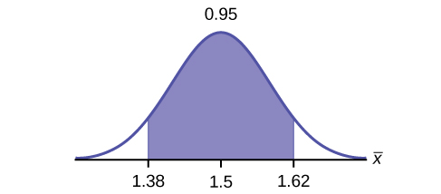
This is a normal distribution curve. The peak of the curve coincides with the point 1.5 on the horizontal axis. A central region is shaded between points 1.38 and 1.62. — Figure 7.9

Solution: EBM = 0.12

e. Explain in complete sentences what the confidence interval means.

3. One hundred eight Americans were surveyed to determine the number of hours they spend watching television each month. It was revealed that they watched an average of 151 hours each month with a standard deviation of 32 hours. Assume that the underlying population distribution is normal.

a. Identify the following:

$\overline{x}$ =_______
${s}_{x}$ =_______
n =_______
n – 1 =_______

Solutions:

$\overline{x}$ = 151
${s}_{x}$ = 32
n = 108
n – 1 = 107

b. Define the random variable X in words.

c. Define the random variable $\overline{x}$ in words.

Solution: $\overline{x}$ is the mean number of hours spent watching television per month from a sample of 108 Americans.

d. Which distribution should you use for this problem?

e. Construct a 99% confidence interval for the population mean hours spent watching television per month. (a) State the confidence interval, (b) sketch the graph, and (c) calculate the error bound.

Solution: CI: (142.92, 159.08)

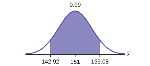
This is a normal distribution curve. The peak of the curve coincides with the point 151 on the horizontal axis. A central region is shaded between points 142.92 and 159.08. — Figure 7.10

Solution: EBM = 8.08

f. Why would the error bound change if the confidence level were lowered to 95%?

4. The data in the table below are the result of a random survey of 39 national flags (with replacement between picks) from various countries. We are interested in finding a confidence interval for the true mean number of colors on a national flag. Let X = the number of colors on a national flag.

Figure 7.11
X	Freq.
1	1
2	7
3	18
4	7
5	6

a. Calculate the following:

$\overline{x}$ =______
${s}_{x}$ =______
n =______

Solutions:

3.26
1.02
39

b. Define the random variable $\overline{x}$ in words.

c. What is $\overline{x}$ estimating?

Solution: μ

d. Is ${\sigma }_{x}$ known?

e. As a result of your answer to the questions above, state the exact distribution to use when calculating the confidence interval.

Solution: t₃₈

f. Construct a 95% confidence interval for the true mean number of colors on national flags. How much area is in both tails (combined)?

g. How much area is in each tail?

Solution: 0.025

h. Calculate the following:

lower limit
upper limit
error bound

i. The 95% confidence interval is_____.

Solution: (2.93, 3.59)

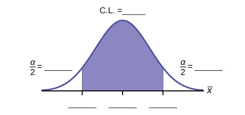
j. Fill in the blanks on the graph with the areas, the upper and lower limits of the Confidence Interval and the sample mean.

This is a template of a normal distribution curve with the central region shaded to represent a confidence interval. The residual areas are on either side of the shaded region. Blanks indicate that students should label the confidence level, residual areas, and points that define the confidence interval. — Figure 7.12

k. In one complete sentence, explain what the interval means.

Solution: We are 95% confident that the true mean number of colors for national flags is between 2.93 colors and 3.59 colors.

l. Using the same $\overline{x}$ , ${s}_{x}$ , and level of confidence, suppose that n were 69 instead of 39. Would the error bound become larger or smaller? How do you know?

Solution: The error bound would become EBM = 0.245. This error bound decreases because as sample sizes increase, variability decreases and we need less interval length to capture the true mean.

m. Using the same $\overline{x}$ , ${s}_{x}$ , and n = 39, how would the error bound change if the confidence level were reduced to 90%? Why?

6. A random survey of enrollment at 35 community colleges across the United States yielded the following figures: 6,414; 1,550; 2,109; 9,350; 21,828; 4,300; 5,944; 5,722; 2,825; 2,044; 5,481; 5,200; 5,853; 2,750; 10,012; 6,357; 27,000; 9,414; 7,681; 3,200; 17,500; 9,200; 7,380; 18,314; 6,557; 13,713; 17,768; 7,493; 2,771; 2,861; 1,263; 7,285; 28,165; 5,080; 11,622. Assume the underlying population is normal.

1. $\overline{x}$ = __________
2. ${s}_{x}$ = __________
3. n = __________
4. n – 1 = __________
Define the random variables $X$ and $\overline{x}$ in words.
Which distribution should you use for this problem? Explain your choice.
Construct a 95% confidence interval for the population mean enrollment at community colleges in the United States.
1. State the confidence interval.
2. Sketch the graph.
3. Calculate the error bound.
What will happen to the error bound and confidence interval if 500 community colleges were surveyed? Why?

Solutions:

1. 8629
2. 6944
3. 35
4. 34
1. CI: (6244, 11,014)
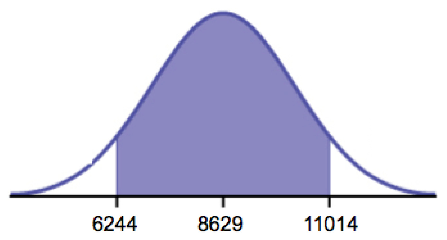
2. Figure 7.13
3. EB = 2385
It will become smaller

7. Suppose that a committee is studying whether or not there is waste of time in our judicial system. It is interested in the mean amount of time individuals waste at the courthouse waiting to be called for jury duty. The committee randomly surveyed 81 people who recently served as jurors. The sample mean wait time was eight hours with a sample standard deviation of four hours.

1. $\overline{x}$ = __________
2. ${s}_{x}$ = __________
3. n = __________
4. n – 1 = __________
Define the random variables $X$ and $\overline{x}$ in words.
Which distribution should you use for this problem? Explain your choice.
Construct a 95% confidence interval for the population mean time wasted.
1. State the confidence interval.
2. Sketch the graph.
3. Calculate the error bound.
Explain in a complete sentence what the confidence interval means.

8. A pharmaceutical company makes tranquilizers. It is assumed that the distribution for the length of time they last is approximately normal. Researchers in a hospital used the drug on a random sample of nine patients. The effective period of the tranquilizer for each patient (in hours) was as follows: 2.7, 2.8, 3.0, 2.3, 2.3, 2.2, 2.8, 2.1, and 2.4.

1. $\overline{x}$ = __________
2. ${s}_{x}$ = __________
3. n = __________
4. n – 1 = __________
Define the random variable $X$ in words.
Define the random variable $\overline{x}$ in words.
Which distribution should you use for this problem? Explain your choice.
Construct a 95% confidence interval for the population mean length of time.
1. State the confidence interval.
2. Sketch the graph.
3. Calculate the error bound.
What does it mean to be “95% confident” in this problem?

Solutions:

1. $\overline{x}$ = 2.51
2. ${s}_{x}$ = 0.318
3. n = 9
4. n – 1 = 8
the effective length of time for a tranquilizer
the mean effective length of time of tranquilizers from a sample of nine patients
We need to use a Student’s-t distribution, because we do not know the population standard deviation.
1. CI: (2.27, 2.76)
2. Check student’s solution.
3. EBM: 0.25
If we were to sample many groups of nine patients, 95% of the samples would contain the true population mean length of time.

9. Suppose that 14 children, who were learning to ride two-wheel bikes, were surveyed to determine how long they had to use training wheels. It was revealed that they used them an average of six months with a sample standard deviation of three months. Assume that the underlying population distribution is normal.

1. $\overline{x}$ = __________
2. ${s}_{x}$ = __________
3. n = __________
4. n – 1 = __________
Define the random variable $X$ in words.
Define the random variable $\overline{x}$ in words.
Which distribution should you use for this problem? Explain your choice.
Construct a 99% confidence interval for the population mean length of time using training wheels.
1. State the confidence interval.
2. Sketch the graph.
3. Calculate the error bound.
Why would the error bound change if the confidence level were lowered to 90%?

10. Forbes magazine published data on the best small firms in 2012. These were firms that had been publicly traded for at least a year, have a stock price of at least $5 per share, and have reported annual revenue between $5 million and $1 billion. The figure below shows the ages of the corporate CEOs for a random sample of these firms.^[2]

Figure 7.14
48	58	51	61	56
59	74	63	53	50
59	60	60	57	46
55	63	57	47	55
57	43	61	62	49
67	67	55	55	49

Use this sample data to construct a 90% confidence interval for the mean age of CEO’s for these top small firms. Use the Student’s t-distribution.

11. Unoccupied seats on flights cause airlines to lose revenue. Suppose a large airline wants to estimate its mean number of unoccupied seats per flight over the past year. To accomplish this, the records of 225 flights are randomly selected and the number of unoccupied seats is noted for each of the sampled flights. The sample mean is 11.6 seats and the sample standard deviation is 4.1 seats.

1. $\overline{x}$ = __________
2. ${s}_{x}$ = __________
3. n = __________
4. n-1 = __________
Define the random variables $X$ and $\overline{x}$ in words.
Which distribution should you use for this problem? Explain your choice.
Construct a 92% confidence interval for the population mean number of unoccupied seats per flight.
1. State the confidence interval.
2. Sketch the graph.
3. Calculate the error bound.

Solutions:

1. $\overline{x}$ = 11.6
2. ${s}_{x}$ = 4.1
3. n = 225
4. n – 1 = 224
X is the number of unoccupied seats on a single flight. $\overline{x}$ is the mean number of unoccupied seats from a sample of 225 flights.
We will use a Student’s-t distribution, because we do not know the population standard deviation.
1. CI: (11.12 , 12.08)
2. Check student’s solution.
3. EBM: 0.48

12. In a recent sample of 84 used car sales costs, the sample mean was $6,425 with a standard deviation of $3,156. Assume the underlying distribution is approximately normal.

Which distribution should you use for this problem? Explain your choice.
Define the random variable $\overline{x}$ in words.
Construct a 95% confidence interval for the population mean cost of a used car.
1. State the confidence interval.
2. Sketch the graph.
3. Calculate the error bound.
Explain what a “95% confidence interval” means for this study.

13. Six different national brands of chocolate chip cookies were randomly selected at the supermarket. The grams of fat per serving are as follows: 8, 8, 10, 7, 9, 9. Assume the underlying distribution is approximately normal.

Construct a 90% confidence interval for the population mean grams of fat per serving of chocolate chip cookies sold in supermarkets.
1. State the confidence interval.
2. Sketch the graph.
3. Calculate the error bound.
If you wanted a smaller error bound while keeping the same level of confidence, what should have been changed in the study before it was done?
Go to the store and record the grams of fat per serving of six brands of chocolate chip cookies.
Calculate the mean.
Is the mean within the interval you calculated in part a? Did you expect it to be? Why or why not?

Solutions:

1. CI: (7.64 , 9.36)
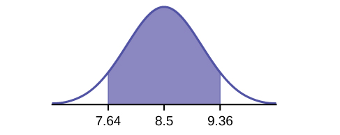
2. Figure 7.15
3. EBM: 0.86
The sample should have been increased.
Answers will vary.
Answers will vary.
Answers will vary.

14. A survey of the mean number of cents off that coupons give was conducted by randomly surveying one coupon per page from the coupon sections of a recent San Jose Mercury News. The following data were collected: 20¢, 75¢, 50¢, 65¢, 30¢, 55¢, 40¢, 40¢, 30¢, 55¢, $1.50, 40¢, 65¢, 40¢.^[3] Assume the underlying distribution is approximately normal.

1. $\overline{x}$ = __________
2. ${s}_{x}$ = __________
3. n = __________
4. n-1 = __________
Define the random variables $X$ and $\overline{x}$ in words.
Which distribution should you use for this problem? Explain your choice.
Construct a 95% confidence interval for the population mean worth of coupons.
1. State the confidence interval.
2. Sketch the graph.
3. Calculate the error bound.
If many random samples were taken of size 14, what percent of the confidence intervals constructed should contain the population mean worth of coupons? Explain why.

15. A quality control specialist for a restaurant chain takes a random sample of size 12 to check the amount of soda served in the 16 oz. serving size. The sample mean is 13.30 with a sample standard deviation of 1.55. Assume the underlying population is normally distributed.

a. Find the 95% Confidence Interval for the true population mean for the amount of soda served.

(12.42, 14.18)
(12.32, 14.29)
(12.50, 14.10)
Impossible to determine

Solution: b

b. What is the error bound?

0.87
1.98
0.99
1.74

12. It is believed that Lake Tahoe Community College (LTCC) Intermediate Algebra students get less than seven hours of sleep per night, on average. A survey of 22 LTCC Intermediate Algebra students generated a mean of 7.24 hours with a standard deviation of 1.93 hours. At a level of significance of 5%, do LTCC Intermediate Algebra students get less than seven hours of sleep per night, on average? The distribution to be used for this test is $\overline{X}$ ~ ________________

$N\left(7.24,\frac{1.93}{\sqrt{22}}\right)$
$N\left(7.24,1.93\right)$
t₂₂
t₂₁

7.3 Sampling Distribution of the Sample Proportion

9. You are performing a hypothesis test of a single population proportion. What must be true about the quantities of np and nq?

Solution: They must both be greater than five.

10. You are performing a hypothesis test of a single population proportion. You find out that np is less than five. What must you do to be able to perform a valid hypothesis test?

11. You are performing a hypothesis test of a single population proportion. The data come from which distribution?

Solution: binomial distribution

7.4 Inference for a Proportion

5. In six packages of “The Flintstones® Real Fruit Snacks” there were five Bam-Bam snack pieces. The total number of snack pieces in the six bags was 68. We wish to calculate a 96% confidence interval for the population proportion of Bam-Bam snack pieces.

Define the random variables X and p̂ in words.
Which distribution should you use for this problem? Explain your choice
Calculate p̂.
Construct a 96% confidence interval for the population proportion of Bam-Bam snack pieces per bag.
1. State the confidence interval.
2. Sketch the graph.
3. Calculate the error bound.
Do you think that six packages of fruit snacks yield enough data to give accurate results? Why or why not?

__________________________?

1. For a class project, a political science student at a large university wants to estimate the percent of students who are registered voters. He surveys 500 students and finds that 300 are registered voters. Compute a 90% confidence interval for the true percent of students who are registered voters, and interpret the confidence interval.

Solution:

x = 300 and n = 500

$\hat{p}=\frac{x}{n}=\frac{300}{500}=0.600$

q‘ = p̂ = 1-0.600 = 0.400

Since CL = 0.90, then α = 1 – CL = 1 – 0.90 = 0.10 $\left(\frac{\alpha }{2}\right)$ = 0.05

${z}_{\frac{\alpha }{2}}$ = z_0.05 = 1.645

$ME=\left({z}_{\frac{\alpha }{2}}\right)\sqrt{\frac{\hat{p}\hat{q}}{n}}=\left(1.645\right)\sqrt{\frac{\left(0.60\right)\left(0.40\right)}{500}}=0.036$

p̂ –ME = 0.60-0.036 = 0.564

p̂ + ME = 0.60+0.036 = 0.636

The confidence interval for the true binomial population proportion is (p̂ – MoE, p̂ + MoE) = (0.564,0.636).

Interpretation:

We estimate with 90% confidence that the true percent of all students that are registered voters is between 56.4% and 63.6%.
Alternate Wording: We estimate with 90% confidence that between 56.4% and 63.6% of ALL students are registered voters.

Explanation of 90% Confidence Level: Ninety percent of all confidence intervals constructed in this way contain the true value for the population percent of students that are registered voters.

2. A student polls his school to see if students in the school district are for or against the new legislation regarding school uniforms. She surveys 600 students and finds that 480 are against the new legislation.

a. Compute a 90% confidence interval for the true percent of students who are against the new legislation, and interpret the confidence interval.

b. In a sample of 300 students, 68% said they own an iPod and a smart phone. Compute a 97% confidence interval for the true percent of students who own an iPod and a smartphone.

3. Marketing companies are interested in knowing the population percent of women who make the majority of household purchasing decisions.

a. When designing a study to determine this population proportion, what is the minimum number you would need to survey to be 90% confident that the population proportion is estimated to within 0.05?

b. If it were later determined that it was important to be more than 90% confident and a new survey were commissioned, how would it affect the minimum number you need to survey? Why?

Solution: It would decrease, because the z-score would decrease, which reducing the numerator and lowering the number.

4. Suppose the marketing company did do a survey. They randomly surveyed 200 households and found that in 120 of them, the woman made the majority of the purchasing decisions. We are interested in the population proportion of households where women make the majority of the purchasing decisions.

a. Identify the following:

x = ______
n = ______
p̂ = ______

b. Define the random variables X and $\hat{p}$ in words.

Solution: X is the number of “successes” where the woman makes the majority of the purchasing decisions for the household.
$\hat{p}$ is the percentage of households sampled where the woman makes the majority of the purchasing decisions for the household.

c. Which distribution should you use for this problem?

You can use the Normal distribution here

d. Construct a 95% confidence interval for the population proportion of households where the women make the majority of the purchasing decisions. State the confidence interval, sketch the graph, and calculate the error bound.

Solution: CI: (0.5321, 0.6679)

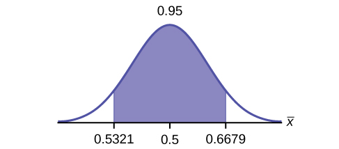
This is a normal distribution curve. The peak of the curve coincides with the point 0.6 on the horizontal axis. A central region is shaded between points 0.5321 and 0.6679. — Figure 7.16

Solution: EBM: 0.0679

e. List two difficulties the company might have in obtaining random results, if this survey were done by email.

5. Of 1,050 randomly selected adults, 360 identified themselves as manual laborers, 280 identified themselves as non-manual wage earners, 250 identified themselves as mid-level managers, and 160 identified themselves as executives. In the survey, 82% of manual laborers preferred trucks, 62% of non-manual wage earners preferred trucks, 54% of mid-level managers preferred trucks, and 26% of executives preferred trucks.

a. We are interested in finding the 95% confidence interval for the percent of executives who prefer trucks. Define random variables X and $\hat{p}$ in words.

Solution: X is the number of “successes” where an executive prefers a truck. $\hat{p}$ is the percentage of executives sampled who prefer a truck.

b. Which distribution should you use for this problem?

You can use the Normal distribution here

c. Construct a 95% confidence interval. State the confidence interval, sketch the graph, and calculate the error bound.

Solution: CI: (0.19432, 0.33068)

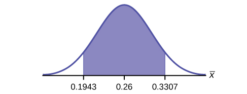
This is a normal distribution curve. The peak of the curve coincides with the point 0.26 on the horizontal axis. A central region is shaded between points 0.1943 and 0.3307. — Figure 7.17

Solution: EBM: 0.0707

d. Suppose we want to lower the sampling error. What is one way to accomplish that?

e. The sampling error given in the survey is ±2%. Explain what the ±2% means.

Solution: The sampling error means that the true mean can be 2% above or below the sample mean.

6. A poll of 1,200 voters asked what the most significant issue was in the upcoming election. Sixty-five percent answered the economy. We are interested in the population proportion of voters who feel the economy is the most important.

a. Define the random variable X in words.

b. Define the random variable $\hat{p}$ in words.

Solution: $\hat{p}$ is the proportion of voters sampled who said the economy is the most important issue in the upcoming election.

c. Which distribution should you use for this problem?

d. Construct a 90% confidence interval, and state the confidence interval and the error bound.

CI: (0.62735, 0.67265)
EBM: 0.02265

e. What would happen to the confidence interval if the level of confidence were 95%?

7. The Ice Chalet offers dozens of different beginning ice-skating classes. All of the class names are put into a bucket. The 5 P.M., Monday night, ages 8 to 12, beginning ice-skating class was picked. In that class were 64 girls and 16 boys. Suppose that we are interested in the true proportion of girls, ages 8 to 12, in all beginning ice-skating classes at the Ice Chalet. Assume that the children in the selected class are a random sample of the population.

a. What is being counted?

The number of girls, ages 8 to 12, in the 5 P.M. Monday night beginning ice-skating class.

b. In words, define the random variable X.

c. Calculate the following:

x = _______
n = _______
p̂ = _______

- x = 64
- n = 80
- p̂ = 0.8

d. State the estimated distribution of X. X~________

e. Define a new random variable $\hat{p}$ . What is p̂ estimating?

p

f. In words, define the random variable $\hat{p}$ .

g. State the estimated distribution of $\hat{p}$ . Construct a 92% Confidence Interval for the true proportion of girls in the ages 8 to 12 beginning ice-skating classes at the Ice Chalet.

$\hat{p}~N\left(0.8,\sqrt{\frac{\left(0.8\right)\left(0.2\right)}{80}}\right)$ . (0.72171, 0.87829).

h. How much area is in both tails (combined)?

i. How much area is in each tail?

0.04

j. Calculate the following:

lower limit
upper limit
error bound

k. The 92% confidence interval is _______.

(0.72; 0.88)

l. Fill in the blanks on the graph with the areas, upper and lower limits of the confidence interval, and the sample proportion.

Normal distribution curve with two vertical upward lines from the x-axis to the curve. The confidence interval is between these two lines. The residual areas are on either side. — Figure 7.18

m. In one complete sentence, explain what the interval means.

With 92% confidence, we estimate the proportion of girls, ages 8 to 12, in a beginning ice-skating class at the Ice Chalet to be between 72% and 88%.

n. Using the same p̂ and level of confidence, suppose that n were increased to 100. Would the error bound become larger or smaller? How do you know?

o. Using the same p̂ and n = 80, how would the error bound change if the confidence level were increased to 98%? Why?

The error bound would increase. Assuming all other variables are kept constant, as the confidence level increases, the area under the curve corresponding to the confidence level becomes larger, which creates a wider interval and thus a larger error.

p. If you decreased the allowable error bound, why would the minimum sample size increase (keeping the same level of confidence)?

8. Insurance companies are interested in knowing the population percent of drivers who always buckle up before riding in a car.

When designing a study to determine this population proportion, what is the minimum number you would need to survey to be 95% confident that the population proportion is estimated to within 0.03?
If it were later determined that it was important to be more than 95% confident and a new survey was commissioned, how would that affect the minimum number you would need to survey? Why?

Solutions:

1,068
The sample size would need to be increased since the critical value increases as the confidence level increases.

Suppose that the insurance companies did do a survey. They randomly surveyed 400 drivers and found that 320 claimed they always buckle up. We are interested in the population proportion of drivers who claim they always buckle up.

1. x = __________
2. n = __________
3. p̂ = __________
Define the random variables X and $\hat{p}$ , in words.
Which distribution should you use for this problem? Explain your choice.
Construct a 95% confidence interval for the population proportion who claim they always buckle up.
1. State the confidence interval.
2. Sketch the graph.
3. Calculate the error bound.
If this survey were done by telephone, list three difficulties the companies might have in obtaining random results.

9. According to a survey of 1,200 people, 61% feel that the president is doing an acceptable job. We are interested in the population proportion of people who feel the president is doing an acceptable job.

Define the random variables X and $\hat{p}$ in words.
Which distribution should you use for this problem? Explain your choice.
Construct a 90% confidence interval for the population proportion of people who feel the president is doing an acceptable job.
1. State the confidence interval.
2. Sketch the graph.
3. Calculate the error bound.

Solutions:

X = the number of people who feel that the president is doing an acceptable job;

P′ = the proportion of people in a sample who feel that the president is doing an acceptable job.
1. CI: (0.59, 0.63)
2. Check student’s solution
3. EBM: 0.02

10. An article regarding interracial dating and marriage appeared in the Washington Post. Of the 1,709 randomly selected adults, 315 identified themselves as Latinos, 323 identified themselves as blacks, 254 identified themselves as Asians, and 779 identified themselves as whites. In this survey, 86% of blacks said that they would welcome a white person into their families. Among Asians, 77% would welcome a white person into their families, 71% would welcome a Latino, and 66% would welcome a black person. ^[4]

We are interested in finding the 95% confidence interval for the percent of all black adults who would welcome a white person into their families. Define the random variables X and $\hat{p}$ , in words.
Which distribution should you use for this problem? Explain your choice.
Construct a 95% confidence interval.
1. State the confidence interval.
2. Sketch the graph.
3. Calculate the error bound.

11. Refer to the information in Number 10.

Construct three 95% confidence intervals.
1. percent of all Asians who would welcome a white person into their families.
2. percent of all Asians who would welcome a Latino into their families.
3. percent of all Asians who would welcome a black person into their families.
Even though the three point estimates are different, do any of the confidence intervals overlap? Which?
For any intervals that do overlap, in words, what does this imply about the significance of the differences in the true proportions?
For any intervals that do not overlap, in words, what does this imply about the significance of the differences in the true proportions?

Solutions:

1. (0.72, 0.82)
2. (0.65, 0.76)
3. (0.60, 0.72)
Yes, the intervals (0.72, 0.82) and (0.65, 0.76) overlap, and the intervals (0.65, 0.76) and (0.60, 0.72) overlap.
We can say that there does not appear to be a significant difference between the proportion of Asian adults who say that their families would welcome a white person into their families and the proportion of Asian adults who say that their families would welcome a Latino person into their families.
We can say that there is a significant difference between the proportion of Asian adults who say that their families would welcome a white person into their families and the proportion of Asian adults who say that their families would welcome a black person into their families.

12. Stanford University conducted a study of whether running is healthy for men and women over age 50. During the first eight years of the study, 1.5% of the 451 members of the 50-Plus Fitness Association died. We are interested in the proportion of people over 50 who ran and died in the same eight-year period.

Define the random variables X and $\hat{p}$ in words.
Which distribution should you use for this problem? Explain your choice.
Construct a 97% confidence interval for the population proportion of people over 50 who ran and died in the same eight–year period.
1. State the confidence interval.
2. Sketch the graph.
3. Calculate the error bound.
Explain what a “97% confidence interval” means for this study.

13. A telephone poll of 1,000 adult Americans was reported in an issue of Time Magazine. One of the questions asked was “What is the main problem facing the country?” Twenty percent answered “crime.”^[5] We are interested in the population proportion of adult Americans who feel that crime is the main problem.

Define the random variables X and $\hat{p}$ in words.
Which distribution should you use for this problem? Explain your choice.
Construct a 95% confidence interval for the population proportion of adult Americans who feel that crime is the main problem.
1. State the confidence interval.
2. Sketch the graph.
3. Calculate the error bound.
Suppose we want to lower the sampling error. What is one way to accomplish that?
The sampling error given by Yankelovich Partners, Inc. (which conducted the poll) is ±3%. In one to three complete sentences, explain what the ±3% represents.

Solutions:

X = the number of adult Americans who feel that crime is the main problem; $\hat{p}$ = the proportion of adult Americans who feel that crime is the main problem
Since we are estimating a proportion, given = 0.2 and n = 1000, the distribution we should use is .
1. CI: (0.18, 0.22)
2. Check student’s solution.
3. EBM: 0.02
One way to lower the sampling error is to increase the sample size.
The stated “± 3%” represents the maximum error bound. This means that those doing the study are reporting a maximum error of 3%. Thus, they estimate the percentage of adult Americans who feel that crime is the main problem to be between 18% and 22%.

14. Refer to the information above. Another question in the poll was “[How much are] you worried about the quality of education in our schools?” Sixty-three percent responded “a lot”. We are interested in the population proportion of adult Americans who are worried a lot about the quality of education in our schools.

Define the random variables X and $\hat{p}$ in words.
Which distribution should you use for this problem? Explain your choice.
Construct a 95% confidence interval for the population proportion of adult Americans who are worried a lot about the quality of education in our schools.
1. State the confidence interval.
2. Sketch the graph.
3. Calculate the error bound.
The sampling error given by Yankelovich Partners, Inc. (which conducted the poll) is ±3%. In one to three complete sentences, explain what the ±3% represents.

15. According to a Field Poll, 79% of California adults (actual results are 400 out of 506 surveyed) feel that “education and our schools” is one of the top issues facing California.^[6] We wish to construct a 90% confidence interval for the true proportion of California adults who feel that education and the schools is one of the top issues facing California.

a. A point estimate for the true population proportion is:

0.90
1.27
0.79
400

Solution: c

b. A 90% confidence interval for the population proportion is _______.

(0.761, 0.820)
(0.125, 0.188)
(0.755, 0.826)
(0.130, 0.183)

c. The error bound is approximately _____.

1.581
0.791
0.059
0.030

Solution: d

16. Five hundred and eleven (511) homes in a certain southern California community are randomly surveyed to determine if they meet minimal earthquake preparedness recommendations. One hundred seventy-three (173) of the homes surveyed met the minimum recommendations for earthquake preparedness, and 338 did not.

a. Find the confidence interval at the 90% Confidence Level for the true population proportion of southern California community homes meeting at least the minimum recommendations for earthquake preparedness.

(0.2975, 0.3796)
(0.6270, 0.6959)
(0.3041, 0.3730)
(0.6204, 0.7025)

b. The point estimate for the population proportion of homes that do not meet the minimum recommendations for earthquake preparedness is ______.

0.6614
0.3386
173
338

Solution: a

17. On May 23, 2013, Gallup reported that of the 1,005 people surveyed, 76% of U.S. workers believe that they will continue working past retirement age. The confidence level for this study was reported at 95% with a ±3% margin of error.^[7]

Determine the estimated proportion from the sample.
Determine the sample size.
Identify CL and α.
Calculate the error bound based on the information provided.
Compare the error bound in part d to the margin of error reported by Gallup. Explain any differences between the values.
Create a confidence interval for the results of this study.
A reporter is covering the release of this study for a local news station. How should she explain the confidence interval to her audience?

18. A national survey of 1,000 adults was conducted on May 13, 2013 by Rasmussen Reports. It concluded with 95% confidence that 49% to 55% of Americans believe that big-time college sports programs corrupt the process of higher education.^[8]

Find the point estimate and the error bound for this confidence interval.
Can we (with 95% confidence) conclude that more than half of all American adults believe this?
Use the point estimate from part a and n = 1,000 to calculate a 75% confidence interval for the proportion of American adults that believe that major college sports programs corrupt higher education.
Can we (with 75% confidence) conclude that at least half of all American adults believe this?

Solutions:

$\hat{p} = \left(\frac{0.55 + 0.49}{2})\right$ = 0.52; MoE = 0.55 – 0.52 = 0.03
No, the confidence interval includes values less than or equal to 0.50. It is possible that less than half of the population believe this.
CL = 0.75, so α = 1 – 0.75 = 0.25 and $\frac{\alpha }{2}=0.125 {z}_{\frac{\alpha }{2}}=1.150$ . (The area to the right of this z is 0.125, so the area to the left is 1 – 0.125 = 0.875.)
$<span style="background-color: #ffffff">MoE</span>=\left(1.150\right)\sqrt{\frac{0.52\left(0.48\right)}{1,000}}\approx 0.018$
(p̂ – MoE, p̂ +MoE) = (0.52 – 0.018, 0.52 + 0.018) = (0.502, 0.538)
Yes – this interval does not fall less than 0.50 so we can conclude that at least half of all American adults believe that major sports programs corrupt education – but we do so with only 75% confidence.

19. Public Policy Polling recently conducted a survey asking adults across the U.S. about music preferences. When asked, 80 of the 571 participants admitted that they have illegally downloaded music.^[9]

Create a 99% confidence interval for the true proportion of American adults who have illegally downloaded music.
This survey was conducted through automated telephone interviews on May 6 and 7, 2013. The error bound of the survey compensates for sampling error, or natural variability among samples. List some factors that could affect the survey’s outcome that are not covered by the margin of error.
Without performing any calculations, describe how the confidence interval would change if the confidence level changed from 99% to 90%.

20. You plan to conduct a survey on your college campus to learn about the political awareness of students. You want to estimate the true proportion of college students on your campus who voted in the 2012 presidential election with 95% confidence and a margin of error no greater than five percent. How many students must you interview?

Solution:

CL = 0.95 α = 1 – 0.95 = 0.05 $\frac{\alpha }{2}$ = 0.025 ${z}_{\frac{\alpha }{2}}$ = 1.96. Use the conservative estimate of $\hat{p}$ = $\hat{q}$ = 0.5.

$n=\frac{ {z}_{\frac{\alpha }{2}}{}^{2}\hat{p}\hat{q}}{MoE}^{2}}= \frac{{1.96}^{2}\left(0.5\right)\left(0.5\right)}{{0.05}^{2}}=384.16$

You need to interview at least 385 students to estimate the proportion to within 5% at 95% confidence.

21. In a recent Zogby International Poll, nine of 48 respondents rated the likelihood of a terrorist attack in their community as “likely” or “very likely.”^[10] Use the “plus four” method to create a 97% confidence interval for the proportion of American adults who believe that a terrorist attack in their community is likely or very likely. Explain what this confidence interval means in the context of the problem.

7.5 Behavior of Confidence Intervals for a Proportion

1. The Berkman Center for Internet & Society at Harvard recently conducted a study analyzing the privacy management habits of teen internet users.^[11] In a group of 50 teens, 13 reported having more than 500 friends on Facebook. Use the “plus four” method to find a 90% confidence interval for the true proportion of teens who would report having more than 500 Facebook friends.

highlight – change to p̂

Solution:

Using “plus-four,” we have x = 13 + 2 = 15 and n = 50 + 4 = 54.

$\hat{p}=\frac{15}{54}\approx 0.278$

$\hat{q}}=1-\hat{p}=1-0.241=0.722$

Since CL = 0.90, we know α = 1 – 0.90 = 0.10 and $\frac{\alpha }{2}$ = 0.05.

${z}_{0.05}=1.645$

$MoE=\left({z}_{\frac{\alpha }{2}}\right)\left(\sqrt{\frac{\hat{p}\hat{q}}{n}}\right)=\left(1.645\right)\left(\sqrt{\frac{\left(0.278\right)\left(0.722\right)}{54}}\right)\approx 0.100$

p̂ – MoE = 0.278 – 0.100 = 0.178

p̂ + MoE = 0.278 + 0.100 = 0.378

We are 90% confident that between 17.8% and 37.8% of all teens would report having more than 500 friends on Facebook

References

Image References

Figure 7.9: Figure 8.13 from OpenStax Introductory Statistics (2013) (CC BY 4.0). Retrieved from https://openstax.org/books/introductory-statistics/pages/8-solutions#eip-589-solution

Figure 7.10: Figure 8.14 from OpenStax Introductory Statistics (2013) (CC BY 4.0). Retrieved from https://openstax.org/books/introductory-statistics/pages/8-solutions#eip-589-solution

Figure 7.12: Figure from Lumen Learning Introduction to Statistics (CC BY 4.0). Retrieved from https://courses.lumenlearning.com/introstats1/chapter/section-exercises-7/

Figure 7.13: Figure 8.20 from OpenStax Introductory Statistics (2013) (CC BY 4.0). Retrieved from https://openstax.org/books/introductory-statistics/pages/8-solutions#eip-589-solution

Figure 7.15: Figure 8.21 from OpenStax Introductory Statistics (2013) (CC BY 4.0). Retrieved from https://openstax.org/books/introductory-statistics/pages/8-solutions#eip-589-solution

Figure 7.16: Figure 8.15 from OpenStax Introductory Statistics (2013) (CC BY 4.0). Retrieved from https://openstax.org/books/introductory-statistics/pages/8-solutions#eip-589-solution

Figure 7.17: Figure 8.16 from OpenStax Introductory Statistics (2013) (CC BY 4.0). Retrieved from https://openstax.org/books/introductory-statistics/pages/8-solutions#eip-589-solution

Figure 7.18: Figure from Lumen Learning Introduction to Statistics (CC BY 4.0). Retrieved from https://courses.lumenlearning.com/introstats1/chapter/section-exercises-7/

Text

“America’s Best Small Companies.” Forbes, 2013. Available online at http://www.forbes.com/best-small-companies/list/ (accessed July 2, 2013).

Data from Microsoft Bookshelf.

Data from http://www.businessweek.com/.

Data from http://www.forbes.com/.

“Disclosure Data Catalog: Leadership PAC and Sponsors Report, 2012.” Federal Election Commission. Available online at http://www.fec.gov/data/index.jsp (accessed July 2,2013).

“Human Toxome Project: Mapping the Pollution in People.” Environmental Working Group. Available online at http://www.ewg.org/sites/humantoxome/participants/participant-group.php?group=in+utero%2Fnewborn (accessed July 2, 2013).

“Metadata Description of Leadership PAC List.” Federal Election Commission. Available online at http://www.fec.gov/finance/disclosure/metadata/metadataLeadershipPacList.shtml (accessed July 2, 2013).

Jensen, Tom. “Democrats, Republicans Divided on Opinion of Music Icons.” Public Policy Polling. Available online at http://www.publicpolicypolling.com/Day2MusicPoll.pdf (accessed July 2, 2013).

Madden, Mary, Amanda Lenhart, Sandra Coresi, Urs Gasser, Maeve Duggan, Aaron Smith, and Meredith Beaton. “Teens, Social Media, and Privacy.” PewInternet, 2013. Available online at http://www.pewinternet.org/Reports/2013/Teens-Social-Media-And-Privacy.aspx (accessed July 2, 2013).

Prince Survey Research Associates International. “2013 Teen and Privacy Management Survey.” Pew Research Center: Internet and American Life Project. Available online at http://www.pewinternet.org/~/media//Files/Questionnaire/2013/Methods%20and%20Questions_Teens%20and%20Social%20Media.pdf (accessed July 2, 2013).

Saad, Lydia. “Three in Four U.S. Workers Plan to Work Past Retirement Age: Slightly more say they will do this by choice rather than necessity.” Gallup® Economy, 2013. Available online at http://www.gallup.com/poll/162758/three-four-workers-plan-work-past-retirement-age.aspx (accessed July 2, 2013).

The Field Poll. Available online at http://field.com/fieldpollonline/subscribers/ (accessed July 2, 2013).

Zogby. “New SUNYIT/Zogby Analytics Poll: Few Americans Worry about Emergency Situations Occurring in Their Community; Only one in three have an Emergency Plan; 70% Support Infrastructure ‘Investment’ for National Security.” Zogby Analytics, 2013. Available online at http://www.zogbyanalytics.com/news/299-americans-neither-worried-nor-prepared-in-case-of-a-disaster-sunyit-zogby-analytics-poll (accessed July 2, 2013).

“52% Say Big-Time College Athletics Corrupt Education Process.” Rasmussen Reports, 2013. Available online at http://www.rasmussenreports.com/public_content/lifestyle/sports/may_2013/52_say_big_time_college_athletics_corrupt_education_process (accessed July 2, 2013).

“Human Toxome Project: Mapping the Pollution in People.” Environmental Working Group. Available online at http://www.ewg.org/sites/humantoxome/participants/participant-group.php?group=in+utero%2Fnewborn (accessed July 2, 2013) ↵
“America’s Best Small Companies.” Forbes, 2013. Available online at http://www.forbes.com/best-small-companies/list/ (accessed July 2, 2013). ↵
Data from San Jose Mercury News ↵
Fears, Darryl., and Deane, Claudia. "Biracial Couples Report Tolerance." Washington Post, July 5, 2001. Available online at https://www.washingtonpost.com/archive/politics/2001/07/05/biracial-couples-report-tolerance/c1ce88c8-ba7c-44f5-a348-b86776df9112. (accessed January 26, 2021). ↵
Data from Time Magazine; survey by Yankelovich Partners, Inc. ↵
The Field Poll. Available online at http://field.com/fieldpollonline/subscribers/ (accessed July 2, 2013). ↵
Saad, Lydia. “Three in Four U.S. Workers Plan to Work Pas Retirement Age: Slightly more say they will do this by choice rather than necessity.” Gallup® Economy, 2013. Available online at http://www.gallup.com/poll/162758/three-fourworkers-plan-work-past-retirement-age.aspx (accessed July 2, 2013). ↵
“52% Say Big-Time College Athletics Corrupt Education Process.” Rasmussen Reports, 2013. Available online at http://www.rasmussenreports.com/public_content/lifestyle/sports/may_2013/ 52_say_big_time_college_athletics_corrupt_education_process (accessed July 2, 2013). ↵
Jensen, Tom. “Democrats, Republicans Divided on Opinion of Music Icons.” Public Policy Polling. Available online at http://www.publicpolicypolling.com/Day2MusicPoll.pdf (accessed July 2, 2013). ↵
Zogby. “New SUNYIT/Zogby Analytics Poll: Few Americans Worry about Emergency Situations Occurring in Their Community; Only one in three have an Emergency Plan; 70% Support Infrastructure ‘Investment’ for National Security.” Zogby Analytics, 2013. Available online at http://www.zogbyanalytics.com/news/299-americans-neither-worried-norprepared-in-case-of-a-disaster-sunyit-zogby-analytics-poll (accessed July 2, 2013). ↵
Prince Survey Research Associates International. “2013 Teen and Privacy Management Survey.” Pew Research Center: Internet and American Life Project. Available online at http://www.pewinternet.org/~/media//Files/Questionnaire/2013/ Methods%20and%20Questions_Teens%20and%20Social%20Media.pdf (accessed July 2, 2013). ↵

License

Icon for the Creative Commons Attribution-ShareAlike 4.0 International License

MATH 1260: Significant Statistics Copyright © 2020 by John Morgan Russell, OpenStaxCollege, OpenIntro is licensed under a Creative Commons Attribution-ShareAlike 4.0 International License, except where otherwise noted.

48	58	51	61	56
59	74	63	53	50
59	60	60	57	46
55	63	57	47	55
57	43	61	62	49
67	67	55	55	49

48	58	51	61	56
59	74	63	53	50
59	60	60	57	46
55	63	57	47	55
57	43	61	62	49
67	67	55	55	49

7.1 Sampling Distribution of the Sample Mean

7.2 Inference for the Mean in Practice

7.3 Sampling Distribution of the Sample Proportion

7.4 Inference for a Proportion

7.5 Behavior of Confidence Intervals for a Proportion

7.1 Sampling Distribution for the Sample Mean

7.2 Inference for the Mean in Practice

7.3 Sampling Distribution of the Sample Proportion

7.4 Inference for a Proportion

7.5 Behavior of Confidence Intervals for a Proportion

7.1 Sampling Distribution for the Sample Mean

7.2 Inference for the Mean in Practice

7.3 Sampling Distribution of the Sample Proportion

7.4 Inference for a Proportion

7.5 Behavior of Confidence Intervals for a Proportion

Image References

Text

License

Share This Book

48	58	51	61	56
59	74	63	53	50
59	60	60	57	46
55	63	57	47	55
57	43	61	62	49
67	67	55	55	49