7.1 The Sampling Distribution of the Sample Mean (σ Un-known)
Learning Objectives
By the end of this chapter, the student should be able to:
- Construct and interpret confidence intervals for means when the population standard deviation is unknown
- Carry out hypothesis tests for means when the population standard deviation is unknown
- Construct and interpret confidence intervals for a proportion
- Understand the behavior of confidence intervals for a proportion
- Carry out hypothesis tests for a proportion
We have discussed the sampling distribution of the sample mean when the population standard deviation, σ, is known. However, in practice, we rarely know the population standard deviation. In the past, when the sample size was large, this did not present a problem to statisticians. They used the sample standard deviation s as an estimate for σ and proceeded as before to calculate a confidence interval with close enough results. However, statisticians ran into problems when the sample size was small. A small sample size can cause inaccuracies in the confidence interval.
Student’s t Distribution

William S. Gosset (1876–1937) of the Guinness brewery in Dublin, Ireland ran into this problem. His experiments with hops and barley produced very few samples. Just replacing σ with s did not always produce accurate results when he tried to use existing inference techniques. He realized that he could not use a normal distribution for the calculation; he found that the actual distribution depends on the sample size. This is because s is a more reliable estimate of σ as samples get bigger. This problem led him to “discover” what is called Student's t-distribution. The name “Student’s T distribution” comes from the fact that Gosset wrote under the pen name “Student.”
Up until the mid-1970s, some statisticians used the normal distribution approximation for large sample sizes and used the Student’s t-distribution only for sample sizes of at most 30. I our current age of technology, the accepted practice now is to simply use the Student’s t-distribution whenever s is used as an estimate for σ.
In summary, if you draw a simple random sample of size n from a population that has an approximately normal distribution with mean μ and unknown population standard deviation σ and calculate the t-score t =  , then the t-scores follow a Student’s t-distribution with n – 1 degrees of freedom. The t-score has the same interpretation as the z-score. It measures how far
  is from its mean μ. For each sample size n, there is a different Student’s t-distribution.
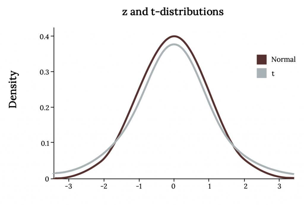
The following images compare the Z (Standard Normal) and t (Student’s T). What differences do you notice?
Degrees of Freedom
The degrees of freedom, n – 1, come from the calculation of the sample standard deviation s. Remember when we calculated a sample standard deviation we divided the sum of the squared deviations by n − 1, but we used n deviations  to calculate s. Because the sum of the deviations is zero, we can find the last deviation once we know the other n – 1 deviations. The other n – 1 deviations can change or vary freely. We call the number n – 1 the degrees of freedom (df).
For example, if we have a sample of size n = 20 items, then we calculate the degrees of freedom as df = n – 1 = 20 – 1 = 19 and we write the distribution as T ~ t19.
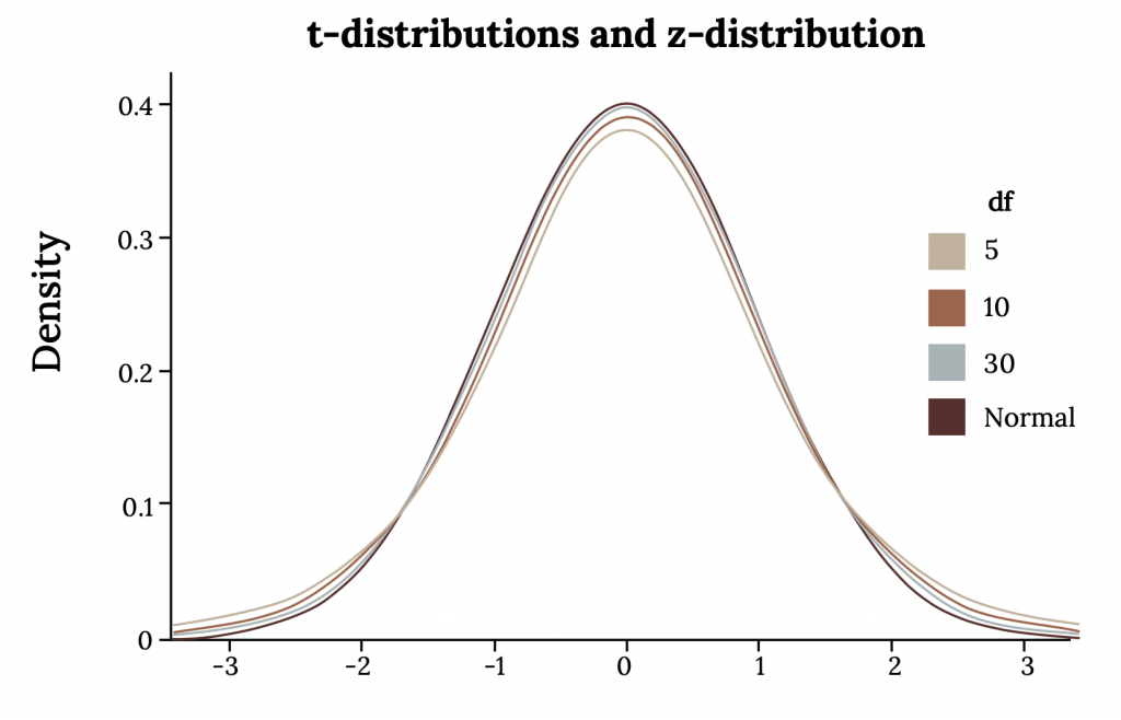
The following image shows what happens to the t distribution as you change the degrees of freedom. What happens as the df increases? What happens once n becomes around 30 and how does that relate to what you already know about the CLT?
Properties of the Student’s t-Distribution
To summarize the properties of the t distribution:
- The graph for the Student’s t-distribution is similar to the standard normal curve, in that it is symmetric about a mean of zero.
- The Student’s t-distribution has more probability in its tails than the standard normal distribution because the spread of the t-distribution is greater than the spread of the standard normal. So the graph of the Student’s t-distribution will be thicker in the tails and shorter in the center than the graph of the standard normal distribution.
- The exact shape of the Student’s t-distribution depends on the degrees of freedom. As the degrees of freedom increases, the graph of Student’s t-distribution becomes more like the graph of the standard normal distribution.
- The underlying population of individual observations is assumed to be normally distributed with unknown population mean μ and unknown population standard deviation σ. The size of the underlying population is generally not relevant unless it is very small. If it is bell shaped (normal) then the assumption is met and doesn’t need discussion. Random sampling is assumed, but that is a completely separate assumption from normality.
- The notation for the Student’s t-distribution (using T as the random variable) is T ~ tdf where df = n – 1.
Example
Suppose you do a study of acupuncture to determine how effective it is in relieving pain. You measure sensory rates for 15 subjects with the results given. Plots of the data show no skewness or outliers. Which distribution is appropriate to use here?
Your turn!
You do a study of hypnotherapy to determine how effective it is in increasing the number of hours of sleep subjects get each night. You measure hours of sleep for 12 subjects and plots of the data show no skewness or outliers. Which distribution is appropriate to use here?
Finding T Distribution Probabilities
A probability table for the Student’s t-distribution can also be used. The table gives t-scores that correspond to the confidence level (column) and degrees of freedom (row). When using a t-table, note that some tables are formatted to show the confidence level in the column headings, while the column headings in some tables may show only corresponding area in one or both tails. Notice that most t tables gives t-scores given the degrees of freedom and the right-tailed probability.
You’ll find that the t table adequate for finding critical values, but is very limited when trying to find p-values. Calculators and computers can easily calculate any Student’s t-probabilities.
Image Credits
Figure 7.1: Phillip Glickman (2019). Public domain. Retrieved from https://unsplash.com/photos/4wnZbnW9Bv0
Figure 7.2: Kindred Grey via Virginia Tech (2021). “Comparing the Standard Normal Distribution and Student’s T Distribution.” CC BY-SA 4.0. Retrieved from https://commons.wikimedia.org/wiki/File:Comparing_the_Standard_Normal_Distribution_and_Student%27s_T_Distribution.png
Figure 7.3: Kindred Grey via Virginia Tech (2021). “T Distribution with Different Degrees of Freedom.” CC BY-SA 4.0. Retrieved from https://commons.wikimedia.org/wiki/File:T_Distribution_with_Different_Degrees_of_Freedom.png
The probability distribution of a statistic at a given sample size
A family of t–distributions, dependent on degrees of freedom, similar to the normal distribution but with more variability built in
The number of objects in a sample that are free to vary
The probability that an event will occur, assuming the null hypothesis is true
