4 Vector Geometry
4.1 Vectors and Lines
In this chapter we study the geometry of 3-dimensional space. We view a point in 3-space as an arrow from the origin to that point. Doing so provides a “picture” of the point that is truly worth a thousand words.
Vectors in 
Introduce a coordinate system in 3-dimensional space in the usual way. First, choose a point  called the
  , then choose three mutually perpendicular lines through , called the
  ,
,  , and
, and  , and establish a number scale on each axis with zero at the origin. Given a point
  in
in  -space we associate three numbers , , and
  with , as described in Figure 4.1.1.
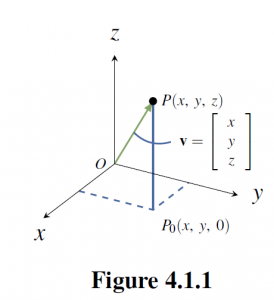
These numbers are called the  of , and we denote the point as
  , or
, or  to emphasize the label . The result is called a
  coordinate system for 3-space, and the resulting description of 3-space is called
  .
.
As in the plane, we introduce vectors by identifying each point with the vector
![\vec{v} = \left[ \begin{array}{c} x \\ y \\ z \end{array} \right]](https://ecampusontario.pressbooks.pub/app/uploads/quicklatex/quicklatex.com-80ba3720048641eb9eba0cf5ad768762_l3.png "Rendered by QuickLaTeX.com") in
in  , represented by the
  from the origin to as in Figure 4.1.1. Informally, we say that the point has vector
  , and that vector has point . In this way 3-space is identified with , and this identification will be made throughout this chapter, often without comment. In particular, the terms “vector” and “point” are interchangeable. The resulting description of 3-space is called
  . Note that the origin is
 ![\vec{0} = \left[ \begin{array}{c} 0 \\ 0 \\ 0 \end{array} \right]](https://ecampusontario.pressbooks.pub/app/uploads/quicklatex/quicklatex.com-30b3e2a1a83469a70aafe843db8bd0fb_l3.png "Rendered by QuickLaTeX.com") .
.
Length and direction
We are going to discuss two fundamental geometric properties of vectors in : length and direction. First, if is a vector with point , the  of vector is defined to be the distance from the origin to , that is the length of the arrow representing . The following properties of length will be used frequently.
Theorem 4.1.1
Let be a vector.
 .
. if and only if
 for all scalars
  .
.
Proof:
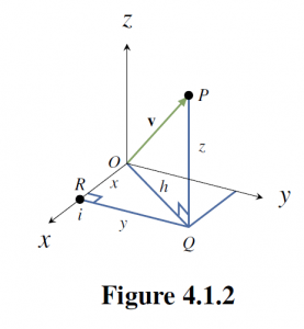
Let have point .
- In Figure 4.1.2,
 is the hypotenuse of the right triangle
  , and so
  by Pythagoras’ theorem. But
  is the hypotenuse of the right triangle
  , so
, so  . Now (1) follows by eliminating
  and taking positive square roots.
 - If
 = 0, then
  by (1). Because squares of real numbers are nonnegative, it follows that
  , and hence that . The converse is because
  .
. - We have
![a\vec{v} = \left[ \begin{array}{ccc} ax & ay & az \end{array}\right]^{T}](https://ecampusontario.pressbooks.pub/app/uploads/quicklatex/quicklatex.com-4ce9697bffaf4a853d6977ba8cc6e4c5_l3.png "Rendered by QuickLaTeX.com") so (1) gives
so (1) gives

Hence
 , and we are done because
  for any real number .
Example 4.1.1
If ![\vec{v} = \left[ \begin{array}{r} 2 \\ -3 \\ 3 \end{array} \right]](https://ecampusontario.pressbooks.pub/app/uploads/quicklatex/quicklatex.com-b4b932d4ab112913c9fc5b4e59fea0d5_l3.png "Rendered by QuickLaTeX.com")
then  . Similarly if
 ![\vec{v} = \left[ \begin{array}{r} 2 \\ -3 \end{array} \right]](https://ecampusontario.pressbooks.pub/app/uploads/quicklatex/quicklatex.com-25f9770c9be4fa3058b6f942fb1b92e5_l3.png "Rendered by QuickLaTeX.com")
in 2-space then  .
.
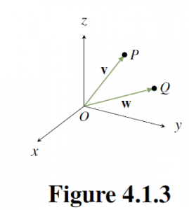
When we view two nonzero vectors as arrows emanating from the origin, it is clear geometrically what we mean by saying that they have the same or opposite  . This leads to a fundamental new description of vectors.
Theorem 4.1.2
Let  and
and  be vectors in . Then
  as matrices if and only if and
  have the same direction and the same length.
Proof:
If , they clearly have the same direction and length. Conversely, let and be vectors with points and  respectively. If and have the same length and direction then, geometrically, and
  must be the same point.
Hence  ,
,  , and
, and  , that is
 ![\vec{v} = \left[ \begin{array}{c} x \\ y \\ z \end{array} \right] = \left[ \begin{array}{c} x_{1} \\ y_{1} \\ z_{1} \end{array} \right] = \vec{w}](https://ecampusontario.pressbooks.pub/app/uploads/quicklatex/quicklatex.com-faeab418ff270d20ea560d22bc4cfd2b_l3.png "Rendered by QuickLaTeX.com") .
.
Note that a vector’s length and direction do  depend on the choice of coordinate system in . Such descriptions are important in applications because physical laws are often stated in terms of vectors, and these laws cannot depend on the particular coordinate system used to describe the situation.
Geometric Vectors
If  and
and  are distinct points in space, the arrow from to has length and direction.
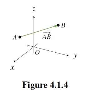
Hence,
Definition 4.1 Geometric vectors
Suppose that and are any two points in . In Figure 4.1.4 the line segment from to is denoted  and is called the
  from to . Point is called the
  of
of  , is called the
  and the is denoted
  .
.
Note that if is any vector in with point then  is itself a geometric vector where is the origin. Referring to as a “vector” seems justified by Theorem 4.1.2 because it has a direction (from to ) and a length . However there appears to be a problem because two geometric vectors can have the same length and direction even if the tips and tails are different.
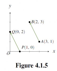
For example and  in Figure 4.1.5 have the same length
  and the same direction (1 unit left and 2 units up) so, by Theorem 4.1.2, they are the same vector! The best way to understand this apparent paradox is to see and as different
  of the same underlying vector
 ![\left[ \begin{array}{r} -1 \\ 2 \end{array} \right]](https://ecampusontario.pressbooks.pub/app/uploads/quicklatex/quicklatex.com-09693e49fe7c8c03aa3c3c5d786849f3_l3.png "Rendered by QuickLaTeX.com") . Once it is clarified, this phenomenon is a great benefit because, thanks to Theorem 4.1.2, it means that the same geometric vector can be positioned anywhere in space; what is important is the length and direction, not the location of the tip and tail. This ability to move geometric vectors about is very useful.
. Once it is clarified, this phenomenon is a great benefit because, thanks to Theorem 4.1.2, it means that the same geometric vector can be positioned anywhere in space; what is important is the length and direction, not the location of the tip and tail. This ability to move geometric vectors about is very useful.
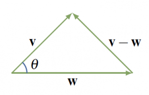
The Parallelogram Law
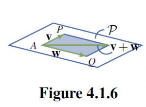
We now give an intrinsic description of the sum of two vectors and in , that is a description that depends only on the lengths and directions of and and not on the choice of coordinate system. Using Theorem 4.1.2 we can think of these vectors as having a common tail . If their tips are and respectively, then they both lie in a plane  containing , , and , as shown in Figure 4.1.6. The vectors and create a parallelogram in , shaded in Figure 4.1.6, called the parallelogram
  by and .
If we now choose a coordinate system in the plane with as origin, then the parallelogram law in the plane shows that their sum  is the diagonal of the parallelogram they determine with tail . This is an intrinsic description of the sum because it makes no reference to coordinates. This discussion proves:
The Parallelogram Law
In the parallelogram determined by two vectors and , the vector is the diagonal with the same tail as and .
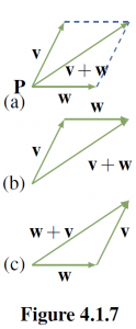
Because a vector can be positioned with its tail at any point, the parallelogram law leads to another way to view vector addition. In Figure 4.1.7 (a) the sum of two vectors and is shown as given by the parallelogram law. If is moved so its tail coincides with the tip of (shown in (b)) then the sum is seen as “first and then . Similarly, moving the tail of to the tip of shows in (c) that is “first and then .” This will be referred to as the  , and it gives a graphic illustration of why
  .
.
Since denotes the vector from a point to a point , the tip-to-tail rule takes the easily remembered form

for any points , , and  .
.
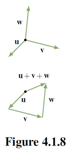
One reason for the importance of the tip-to-tail rule is that it means two or more vectors can be added by placing them tip-to-tail in sequence. This gives a useful “picture” of the sum of several vectors, and is illustrated for three vectors in Figure 4.1.8 where  is viewed as first
  , then , then .
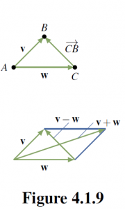
There is a simple geometrical way to visualize the (matrix) 
 of two vectors. If and are positioned so that they have a common tail , and if and are their respective tips, then the tip-to-tail rule gives
  . Hence
  is the vector from the tip of to the tip of . Thus both and appear as diagonals in the parallelogram determined by and (see Figure 4.1.9.
Theorem 4.1.3
If and have a common tail, then is the vector from the tip of to the tip of .
One of the most useful applications of vector subtraction is that it gives a simple formula for the vector from one point to another, and for the distance between the points.
Theorem 4.1.4
Let  and
and  be two points. Then:
![\vec{P_{1}P}_{2} = \left[ \begin{array}{c} x_{2} - x_{1} \\ y_{2} - y_{1} \\ z_{2} - z_{1} \end{array} \right]](https://ecampusontario.pressbooks.pub/app/uploads/quicklatex/quicklatex.com-0d91b62f61e2ab368818c961ede56673_l3.png "Rendered by QuickLaTeX.com") .
.- The distance between
 and
and  is
is 
Can you prove these results?
Example 4.1.3
The distance between  and
and  is
is  , and the vector from to is
![\vec{P_{1}P}_{2} = \left[ \begin{array}{r} -1 \\ 2 \\ 1 \end{array} \right]](https://ecampusontario.pressbooks.pub/app/uploads/quicklatex/quicklatex.com-4f11ea97f1984fb31df5e2ab319e7104_l3.png "Rendered by QuickLaTeX.com") .
.
The next theorem tells us what happens to the length and direction of a scalar multiple of a given vector.
Scalar Multiple Law
If a is a real number and is a vector then:
- The length of
 is
is  .
. - If
 , the direction of is the same as if
  ; opposite to if
Proof:
The first statement is true due to Theorem 4.1.1.
To prove the second statement, let denote the origin in  Let have point , and choose any plane containing and . If we set up a coordinate system in this plane with as origin, then so the result follows from the scalar multiple law in the plane.
A vector is called a  if
if  . Then
![\vec{i} = \left[ \begin{array}{c} 1 \\ 0 \\ 0 \end{array} \right]](https://ecampusontario.pressbooks.pub/app/uploads/quicklatex/quicklatex.com-f4675ab4908dccc00c63fa4377ec2134_l3.png "Rendered by QuickLaTeX.com") ,
, ![\vec{j} = \left[ \begin{array}{c} 0 \\ 1 \\ 0 \end{array} \right]](https://ecampusontario.pressbooks.pub/app/uploads/quicklatex/quicklatex.com-247115bfd0abd328188d22d4d7729d86_l3.png "Rendered by QuickLaTeX.com") , and
, and ![\vec{k} = \left[ \begin{array}{c} 0 \\ 0 \\ 1 \end{array} \right]](https://ecampusontario.pressbooks.pub/app/uploads/quicklatex/quicklatex.com-6b34f73e2b2c16fd6b2cda1d7ece4bf0_l3.png "Rendered by QuickLaTeX.com")
are unit vectors, called the  vectors.
Example 4.1.4
If show that  is the unique unit vector in the same direction as
Solution:
The vectors in the same direction as are the scalar multiples where  . But
. But  when , so is a unit vector if and only if
  .
.
Definition 4.2 Parallel vectors in
Two nonzero vectors are called  if they have the same or opposite direction.
Theorem 4.1.5
Two nonzero vectors and are parallel if and only if one is a scalar multiple of the other.
Example 4.1.5
Given points  ,
,  ,
,  , and
, and  , determine if and are parallel.
Solution:
By Theorem 4.1.3,  and
and  . If
. If 
then  , so
, so  and
and  , which is impossible. Hence is a scalar multiple of , so these vectors are not parallel by Theorem 4.1.5.
Lines in Space
These vector techniques can be used to give a very simple way of describing straight lines in space. In order to do this, we first need a way to
specify the orientation of such a line.
Definition 4.3 Direction Vector of a Line
We call a nonzero vector  a direction vector for the line if it is parallel to for some pair of distinct points and on the line.
Note that any nonzero scalar multiple of  would also serve as a direction vector of the line.
We use the fact that there is exactly one line that passes through a particular point  and has a given direction vector
![\vec{d} = \left[ \begin{array}{c} a \\ b \\ c \end{array} \right]](https://ecampusontario.pressbooks.pub/app/uploads/quicklatex/quicklatex.com-ec3f3226d3e1112c9896e325903c769f_l3.png "Rendered by QuickLaTeX.com") . We want to describe this line by giving a condition on , , and that the point lies on this line. Let
. We want to describe this line by giving a condition on , , and that the point lies on this line. Let
![\vec{p}_{0} = \left[ \begin{array}{c} x_{0} \\ y_{0} \\ z_{0} \end{array} \right]](https://ecampusontario.pressbooks.pub/app/uploads/quicklatex/quicklatex.com-6ad903adbe0411494705af4e8f5ef084_l3.png "Rendered by QuickLaTeX.com")
and ![\vec{p} = \left[ \begin{array}{c} x \\ y \\ z \end{array} \right]](https://ecampusontario.pressbooks.pub/app/uploads/quicklatex/quicklatex.com-94351a7c5397f16180d12b7ac8619c8c_l3.png "Rendered by QuickLaTeX.com") denote the vectors of
denote the vectors of  and , respectively.
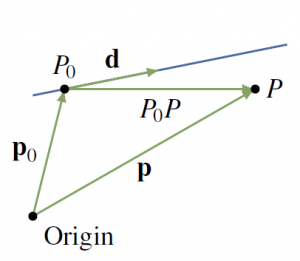
Then

Hence lies on the line if and only if  is parallel to —that is, if and only if
  for some scalar
  by Theorem 4.1.5. Thus
  is the vector of a point on the line if and only if
  for some scalar .
Vector Equation of a line
The line parallel to through the point with vector  is given by

In other words, the point with vector is on this line if and only if a real number t exists such that .
In component form the vector equation becomes
![\begin{equation*} \left[ \begin{array}{c} x \\ y \\ z \end{array} \right] = \left[ \begin{array}{c} x_{0} \\ y_{0} \\ z_{0} \end{array} \right] + t \left[ \begin{array}{c} a \\ b \\ c \end{array} \right] \end{equation*}](https://ecampusontario.pressbooks.pub/app/uploads/quicklatex/quicklatex.com-913ee00b2bc4988c7904bf047f87fc13_l3.png "Rendered by QuickLaTeX.com")
Equating components gives a different description of the line.
Parametric Equations of a line
The line through with direction vector
![\vec{d} = \left[ \begin{array}{c} a \\ b \\ c \end{array} \right] \neq \vec{0}](https://ecampusontario.pressbooks.pub/app/uploads/quicklatex/quicklatex.com-28eca1be57947254a98ec01d662baab9_l3.png "Rendered by QuickLaTeX.com") is given by
is given by

In other words, the point is on this line if and only if a real number exists such that  ,
,  , and
, and  .
.
Example 4.1.6
Find the equations of the line through the points  and
and  .
.
Solution:
Let
![\vec{d} = \vec{P_{0}P}_{1} = \left[ \begin{array}{c} 2 \\ 1 \\ 0 \end{array} \right]](https://ecampusontario.pressbooks.pub/app/uploads/quicklatex/quicklatex.com-4810a1f6d35bb92109008d73ff2d7f2a_l3.png "Rendered by QuickLaTeX.com")
denote the vector from to . Then is parallel to the line ( and are on the line), so serves as a direction vector for the line. Using as the point on the line leads to the parametric equations

Note that if is used (rather than ), the equations are

These are different from the preceding equations, but this is merely the result of a change of parameter. In fact,  .
.
Example 4.1.7
Determine whether the following lines intersect and, if so, find the point of intersection.

Solution:
Suppose with vector lies on both lines. Then
![\begin{equation*} \left[ \begin{array}{c} 1 - 3t \\ 2 + 5t \\ 1 + t \end{array} \right] = \left[ \begin{array}{c} x \\ y \\ z \end{array} \right] = \left[ \begin{array}{c} -1 + s \\ 3 - 4s \\ 1 - s \end{array} \right] \mbox{ for some } t \mbox{ and } s, \end{equation*}](https://ecampusontario.pressbooks.pub/app/uploads/quicklatex/quicklatex.com-f905eedb03545c1d8a45db08b6ebeef6_l3.png "Rendered by QuickLaTeX.com")
where the first (second) equation is because lies on the first (second) line. Hence the lines intersect if and only if the three equations

have a solution. In this case,  and
and  satisfy all three equations, so the lines do intersect and the point of intersection is
![\begin{equation*} \vec{p} = \left[ \begin{array}{c} 1 - 3t \\ 2 + 5t \\ 1 + t \end{array} \right] = \left[ \begin{array}{r} -2 \\ 7 \\ 2 \end{array} \right] \end{equation*}](https://ecampusontario.pressbooks.pub/app/uploads/quicklatex/quicklatex.com-0040d1e22ad92cc9b05a2e7d53180ef3_l3.png "Rendered by QuickLaTeX.com")
using . Of course, this point can also be found from
![\vec{p} = \left[ \begin{array}{c} -1 + s \\ 3 - 4s \\ 1 - s \end{array} \right]](https://ecampusontario.pressbooks.pub/app/uploads/quicklatex/quicklatex.com-4d91258eaf2175b078cb37691b1d8fa5_l3.png "Rendered by QuickLaTeX.com") using .
using .
4.2 Projections and Planes
Suppose a point and a plane are given and it is desired to find the point that lies in the plane and is closest to , as shown in Figure 4.2.1.
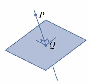
Clearly, what is required is to find the line through that is perpendicular to the plane and then to obtain as the point of intersection of this line with the plane. Finding the line perpendicular to the plane requires a way to determine when two vectors are perpendicular. This can be done using the idea of the dot product of two vectors.
The Dot Product and Angles
Definition 4.4 Dot Product in 
Given vectors
![\vec{v} = \left[ \begin{array}{c} x_{1} \\ y_{1}\\ z_{1} \end{array} \right]](https://ecampusontario.pressbooks.pub/app/uploads/quicklatex/quicklatex.com-ccc7d26a8ee7d698dd1d48eaefd0f0e5_l3.png "Rendered by QuickLaTeX.com") and
and
![\vec{w} = \left[ \begin{array}{c} x_{2} \\ y_{2}\\ z_{2} \end{array} \right]](https://ecampusontario.pressbooks.pub/app/uploads/quicklatex/quicklatex.com-70280013eed5b9fc9490c20eeaeb7542_l3.png "Rendered by QuickLaTeX.com") , their dot product
, their dot product  is a number defined

Because  is a number, it is sometimes called the scalar product of and
Example 4.2.1
If ![\vec{v} = \left[ \begin{array}{r} 2 \\ -1 \\ 3 \end{array} \right]](https://ecampusontario.pressbooks.pub/app/uploads/quicklatex/quicklatex.com-7c0f43e3bdf79d6d2cce2b685b867aaa_l3.png "Rendered by QuickLaTeX.com")
and ![\vec{w} = \left[ \begin{array}{r} 1 \\ 4\\ -1 \end{array} \right]](https://ecampusontario.pressbooks.pub/app/uploads/quicklatex/quicklatex.com-4fe5be9b5f6bc750aac3b0ef910233fa_l3.png "Rendered by QuickLaTeX.com") , then
, then  .
.
Theorem 4.2.1
Let , , and denote vectors in (or  ).
).
- is a real number.
 .
. .
. .
. for all scalars
  .
.
The readers are invited to prove these properties using the definition of dot products.
Example 4.2.2
Verify that  when
when  ,
,  , and
, and  .
.
Solution:
We apply Theorem 4.2.1 several times:

There is an intrinsic description of the dot product of two nonzero vectors in  . To understand it we require the following result from trigonometry.
Laws of Cosine
If a triangle has sides ,  , and
, and  , and if
  is the interior angle opposite then

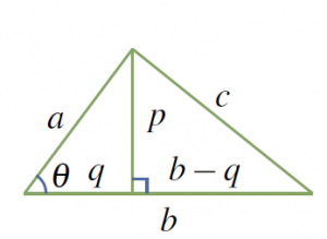
Proof:
We prove it when is acute, that is  ; the obtuse case is similar. In Figure 4.2.2 we have
  and
and  .
.
Hence Pythagoras’ theorem gives

The law of cosines follows because  for any angle .
Note that the law of cosines reduces to Pythagoras’ theorem if is a right angle (because  ).
).
Now let and be nonzero vectors positioned with a common tail. Then they determine a unique angle in the range

This angle will be called the angle between and . Clearly  and
and  are parallel if is either
  or
or  . Note that we do not define the angle between and if one of these vectors is
  .
.
The next result gives an easy way to compute the angle between two nonzero vectors using the dot product.
Theorem 4.2.2
Let and be nonzero vectors. If is the angle between and , then

Proof:
We calculate  in two ways. First apply the law of cosines to the triangle in Figure 4.2.4 to obtain:

On the other hand, we use Theorem 4.2.1:

Comparing these we see that  , and the result follows.
If and are nonzero vectors, Theorem 4.2.2 gives an intrinsic description of because ,  , and the angle between and do not depend on the choice of coordinate system. Moreover, since and
  are nonzero ( and are nonzero vectors), it gives a formula for the cosine of the angle :

Since  , this can be used to find .
Example 4.2.3
Compute the angle between
![\vec{u} = \left[ \begin{array}{r} -1 \\ 1 \\ 2 \end{array} \right]](https://ecampusontario.pressbooks.pub/app/uploads/quicklatex/quicklatex.com-93f90b07b74ac41fc0efde25cb24acca_l3.png "Rendered by QuickLaTeX.com") and
and
![\vec{v} = \left[ \begin{array}{r} 2 \\ 1 \\ -1 \end{array} \right]](https://ecampusontario.pressbooks.pub/app/uploads/quicklatex/quicklatex.com-2688c17ee8f7b48b529b8e9c5c0ce619_l3.png "Rendered by QuickLaTeX.com") .
.
Solution:
Compute  . Now recall that
  and
and  are defined so that (
 , ) is the point on the unit circle determined by the angle (drawn counterclockwise, starting from the positive axis). In the present case, we know that
  and that . Because
  , it follows that
  .
.
If and are nonzero, the previous example shows that has the same sign as  , so
, so

In this last case, the (nonzero) vectors are perpendicular. The following terminology is used in linear algebra:
Definition 4.5 Orthogonal Vectors in
Two vectors and are said to be \textbf{orthogonal}\index{orthogonal vectors}\index{vectors!orthogonal vectors} if  or
or  or the angle between them is
  .
.
Since  if either or
  , we have the following theorem:
Theorem 4.2.3
Two vectors and are orthogonal if and only if .
Example 4.2.4
Show that the points  ,
,  , and
, and  are the vertices of a right triangle.
Solution:
The vectors along the sides of the triangle are
![\begin{equation*} \vec{PQ} = \left[ \begin{array}{r} 1 \\ 2 \\ 3 \end{array} \right],\ \vec{PR} = \left[ \begin{array}{r} 3 \\ 1 \\ 3 \end{array} \right], \mbox{ and } \vec{QR} = \left[ \begin{array}{r} 2 \\ -1 \\ 0 \end{array} \right] \end{equation*}](https://ecampusontario.pressbooks.pub/app/uploads/quicklatex/quicklatex.com-3e3b1c1d081b9ec86e5528232093cf76_l3.png "Rendered by QuickLaTeX.com")
Evidently  , so and
  are orthogonal vectors. This means sides
  and
and  are perpendicular—that is, the angle at is a right angle.
Projections
In applications of vectors, it is frequently useful to write a vector as the sum of two orthogonal vectors.
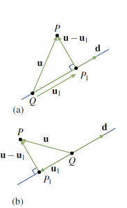
If a nonzero vector is specified, the key idea is to be able to write an arbitrary vector as a sum of two vectors,

where  is parallel to and
  is orthogonal to . Suppose that and emanate from a common tail (see Figure 4.2.5). Let be the tip of , and let denote the foot of the perpendicular from to the line through parallel to .
Then  has the required properties:
1. is parallel to .
2. is orthogonal to .
3.  .
.
Definition 4.6 Projection in
The vector in Figure 4.2.6 is called the projection of on .
It is denoted

In Figure 4.2.5 (a) the vector  has the same direction as ; however, and have opposite directions if the angle between and is greater than (see Figure 4.2.5 (b)). Note that the projection
  is zero if and only if and are orthogonal.
Calculating the projection of on is remarkably easy.
Theorem 4.2.4
Let and be vectors.
- The projection of on is given by
 .
. - The vector
 is orthogonal to .
Proof:
The vector is parallel to and so has the form  for some scalar . The requirement that
  and are orthogonal determines . In fact, it means that
  by Theorem 4.2.3. If is substituted here, the condition is

It follows that  , where the assumption that guarantees that
  .
.
Example 4.2.5
Find the projection of
![\vec{u} = \left[ \begin{array}{r} 2 \\ -3 \\ 1 \end{array} \right]](https://ecampusontario.pressbooks.pub/app/uploads/quicklatex/quicklatex.com-0bb860cb56cb147d36cb34352a55bf1f_l3.png "Rendered by QuickLaTeX.com")
on ![\vec{d} = \left[ \begin{array}{r} 1\\ -1 \\ 3 \end{array} \right]](https://ecampusontario.pressbooks.pub/app/uploads/quicklatex/quicklatex.com-7c1cfdacba1089d8c65ea6ff7c57b9aa_l3.png "Rendered by QuickLaTeX.com")
and express where is parallel to and  is orthogonal to .
Solution:
The projection of on is
![\begin{equation*} \vec{u}_{1} = proj_{\vec{d}}{\vec{u}} = \frac{\vec{u} \cdot \vec{d}}{|| \vec{d}|| ^2}\vec{d} = \frac{2 + 3 + 3}{1^2 + (-1)^2 + 3^2} \left[ \begin{array}{r} 1\\ -1 \\ 3 \end{array} \right] = \frac{8}{11}\left[ \begin{array}{r} 1\\ -1 \\ 3 \end{array} \right] \end{equation*}](https://ecampusontario.pressbooks.pub/app/uploads/quicklatex/quicklatex.com-229e18f2b977031aa3cad7ce46bd7fa9_l3.png "Rendered by QuickLaTeX.com")
Hence ![\vec{u}_{2} = \vec{u} - \vec{u}_{1} = \frac{1}{11}\left[ \begin{array}{r} 14\\ -25 \\ -13 \end{array} \right]](https://ecampusontario.pressbooks.pub/app/uploads/quicklatex/quicklatex.com-d355e039a801512cbfd7c8d63343162c_l3.png "Rendered by QuickLaTeX.com") , and this is orthogonal to by Theorem 4.2.4 (alternatively, observe that
, and this is orthogonal to by Theorem 4.2.4 (alternatively, observe that  ). Since , we are done.
Note that the idea of projections can be used to find the shortest distance from a point to a straight line in  which is
  the length of the vector that’s orthogonal to the direction vector of the line.
Planes
Definition 4.7 Normal vector in a plane
A nonzero vector  is called a normal for a plane if it is orthogonal to every vector in the plane.
For example, the unit vector  is a normal vector for
  plane.
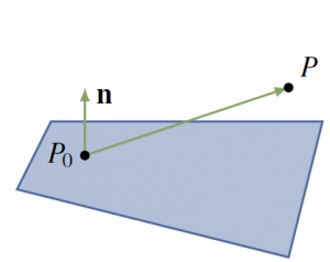
Given a point  and a nonzero vector , there is a unique plane through with normal , shaded in Figure 4.2.6. A point
  lies on this plane if and only if the vector is orthogonal to —that is, if and only if
  . Because
 ![\vec{P_{0}P} = \left[ \begin{array}{c} x - x_{0}\\ y - y_{0}\\ z - z_{0} \end{array} \right]](https://ecampusontario.pressbooks.pub/app/uploads/quicklatex/quicklatex.com-040991c9a930deb0cdd53f9c03415336_l3.png "Rendered by QuickLaTeX.com") this gives the following result:
this gives the following result:
Scalar equation of a plane
The plane through with normal ![\vec{n} = \left[ \begin{array}{c} a\\ b\\ c \end{array} \right] \neq \vec{0}](https://ecampusontario.pressbooks.pub/app/uploads/quicklatex/quicklatex.com-e540d456bec740c05b4756a0ab40cd78_l3.png "Rendered by QuickLaTeX.com")
as a normal vector is given by

In other words, a point is on this plane if and only if , , and satisfy this equation.
Example 4.2.8
Find an equation of the plane through  with
with ![\vec{n} = \left[ \begin{array}{r} 3\\ -1\\ 2 \end{array} \right]](https://ecampusontario.pressbooks.pub/app/uploads/quicklatex/quicklatex.com-c31b123472f9ceb8db8d5c77336438fd_l3.png "Rendered by QuickLaTeX.com")
as normal.
Solution:
Here the general scalar equation becomes

This simplifies to  .
.
If we write  , the scalar equation shows that every plane with normal
 ![\vec{n} = \left[ \begin{array}{r} a\\ b\\ c \end{array} \right]](https://ecampusontario.pressbooks.pub/app/uploads/quicklatex/quicklatex.com-340e85cba46b65e1ad25f1c96d8506b3_l3.png "Rendered by QuickLaTeX.com")
has a linear equation of the form
(4.2) 
for some constant  . Conversely, the graph of this equation is a plane with as a normal vector (assuming that , , and are not all zero).
Example 4.2.9
Find an equation of the plane through  that is parallel to the plane with equation
  .
.
Solution:
The plane with equation  has normal
 ![\vec{n} = \left[ \begin{array}{r} 2\\ -3\\ 0 \end{array} \right]](https://ecampusontario.pressbooks.pub/app/uploads/quicklatex/quicklatex.com-f020d7732719774ab8206fbfc6258558_l3.png "Rendered by QuickLaTeX.com") . Because the two planes are parallel, serves as a normal for the plane we seek, so the equation is
. Because the two planes are parallel, serves as a normal for the plane we seek, so the equation is  for some according to (4.2). Insisting that lies on the plane determines ; that is,
  . Hence, the equation is
  .
.
Consider points and with vectors ![\vec{p}_{0} = \left[ \begin{array}{r} x_{0}\\ y_{0}\\ z_{0} \end{array} \right]](https://ecampusontario.pressbooks.pub/app/uploads/quicklatex/quicklatex.com-3e5c0f59df06ae7ce9eb83f8ca01bd2e_l3.png "Rendered by QuickLaTeX.com")
and
![\vec{p}= \left[ \begin{array}{r} x\\ y\\ z \end{array} \right]](https://ecampusontario.pressbooks.pub/app/uploads/quicklatex/quicklatex.com-e5424f262d9670b35e3c6d66211089ca_l3.png "Rendered by QuickLaTeX.com") .
.
Given a nonzero vector , the scalar equation of the plane through with normal takes the vector form:
Vector Equation of a Plane
The plane with normal  through the point with vector is given by

In other words, the point with vector is on the plane if and only if satisfies this condition.
Moreover, Equation (4.2) translates as follows:
Every plane with normal has vector equation  for some number .
Example 4.2.10
Find the shortest distance from the point  to the plane with equation
  . Also find the point on this plane closest to .
Solution:
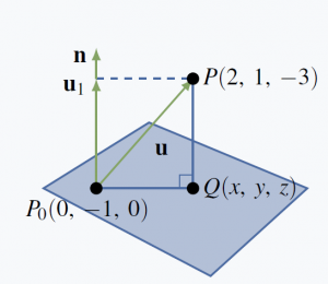 The plane in question has normal
 ![\vec{n} = \left[ \begin{array}{r} 3\\ -1\\ 4 \end{array} \right]](https://ecampusontario.pressbooks.pub/app/uploads/quicklatex/quicklatex.com-9eddd17b93bab1d235644038f04f8744_l3.png "Rendered by QuickLaTeX.com") . Choose any point on the plane—say
. Choose any point on the plane—say  —and let
  be the point on the plane closest to (see the diagram). The vector from to is
 ![\vec{u} = \left[ \begin{array}{r} 2\\ 2\\ -3 \end{array} \right]](https://ecampusontario.pressbooks.pub/app/uploads/quicklatex/quicklatex.com-35fb49d4e5f82dbbb7e07c7de46efa13_l3.png "Rendered by QuickLaTeX.com") . Now erect with its tail at . Then
. Now erect with its tail at . Then  and is the projection of on :
![\begin{equation*} \vec{u}_{1} = \frac{\vec{n} \cdot \vec{u}}{|| \vect{n} ||^2}\vec{n} = \frac{-8}{26} \left[ \begin{array}{r} 3\\ -1 \\ 4 \end{array} \right] = \frac{-4}{13} \left[ \begin{array}{r} 3\\ -1 \\ 4 \end{array} \right] \end{equation*}](https://ecampusontario.pressbooks.pub/app/uploads/quicklatex/quicklatex.com-9aa0e384b6ac6a0869df3536cb19614e_l3.png "Rendered by QuickLaTeX.com")
Hence the distance is  . To calculate the point , let
 ![\vec{q} = \left[ \begin{array}{r} x\\ y \\ z \end{array} \right]](https://ecampusontario.pressbooks.pub/app/uploads/quicklatex/quicklatex.com-416977fffd2455e19a6748c0b6c8ed8a_l3.png "Rendered by QuickLaTeX.com")
and
![\vec{p}_{0} = \left[ \begin{array}{r} 0\\ -1 \\ 0 \end{array} \right]](https://ecampusontario.pressbooks.pub/app/uploads/quicklatex/quicklatex.com-3ac66f3bc93a4bac9339ea0ff5e49023_l3.png "Rendered by QuickLaTeX.com")
be the vectors of and . Then
![\begin{equation*} \vec{q} = \vec{p}_{0} + \vec{u} - \vec{u}_{1} = \left[ \begin{array}{r} 0\\ -1 \\ 0 \end{array} \right] + \left[ \begin{array}{r} 2\\ 2 \\ -3 \end{array} \right] + \frac{4}{13} \left[ \begin{array}{r} 3\\ -1 \\ 4 \end{array} \right] = \left[ \def\arraystretch{1.5} \begin{array}{r} \frac{38}{13}\\ \frac{9}{13}\\ \frac{-23}{13} \end{array} \right] \end{equation*}](https://ecampusontario.pressbooks.pub/app/uploads/quicklatex/quicklatex.com-5ed3cb7c5cbb20c5768fbebb04639a1c_l3.png "Rendered by QuickLaTeX.com")
This gives the coordinates of  .
.
The Cross Product
If , , and  are three distinct points in that are not all on some line, it is clear geometrically that there is a unique plane containing all three. The vectors
  and
and  both lie in this plane, so finding a normal amounts to finding a nonzero vector orthogonal to both and . The cross product provides a systematic way to do this.
Definition 4.8 Cross Product
Given vectors ![\vec{v}_{1}= \left[ \begin{array}{c} x_{1}\\ y_{1} \\ z_{1} \end{array} \right]](https://ecampusontario.pressbooks.pub/app/uploads/quicklatex/quicklatex.com-7c902e8ce90cec9925616cca68a10db5_l3.png "Rendered by QuickLaTeX.com") and
and ![\vec{v}_{2}= \left[ \begin{array}{c} x_{2}\\ y_{2} \\ z_{2} \end{array} \right]](https://ecampusontario.pressbooks.pub/app/uploads/quicklatex/quicklatex.com-0d49b1281bfe537b3ad0d7549ed2cd6a_l3.png "Rendered by QuickLaTeX.com") , define the cross product
, define the cross product  by
by
![\begin{equation*} \vec{v}_{1} \times \vec{v}_{2} = \left[ \begin{array}{c} y_{1}z_{2} - z_{1}y_{2}\\ -(x_{1}z_{2} - z_{1}x_{2}) \\ x_{1}y_{2} - y_{1}x_{2} \end{array} \right] \end{equation*}](https://ecampusontario.pressbooks.pub/app/uploads/quicklatex/quicklatex.com-55cbd31ea43058baf071509d0a2c06fc_l3.png "Rendered by QuickLaTeX.com")
Because it is a vector, is often called the vector product. There is an easy way to remember this definition using the coordinate vectors:
![\begin{equation*} \vec{i}= \left[ \begin{array}{c} 1\\ 0 \\ 0 \end{array} \right], \ \vec{j}= \left[ \begin{array}{c} 0\\ 1 \\ 0 \end{array} \right], \mbox{ and } \vec{k}= \left[ \begin{array}{c} 0\\ 0 \\ 1 \end{array} \right] \end{equation*}](https://ecampusontario.pressbooks.pub/app/uploads/quicklatex/quicklatex.com-43da99f15cba2c717daf5a63ae84072f_l3.png "Rendered by QuickLaTeX.com")
They are vectors of length  pointing along the positive , , and axes. The reason for the name is that any vector can be written as
![\begin{equation*} \left[ \begin{array}{c} x\\ y \\ z \end{array} \right] = x\vec{i} + y\vec{j} + z\vec{k} \end{equation*}](https://ecampusontario.pressbooks.pub/app/uploads/quicklatex/quicklatex.com-562d5b6ec1553207d7c2bae68bdf340b_l3.png "Rendered by QuickLaTeX.com")
With this, the cross product can be described as follows:
Determinant form of the cross product
If ![\vec{v}_{1}= \left[ \begin{array}{c} x_{1}\\ y_{1}\\ z_{1} \end{array} \right]](https://ecampusontario.pressbooks.pub/app/uploads/quicklatex/quicklatex.com-2f8993b9aa1dc1aeab91d719ff148d81_l3.png "Rendered by QuickLaTeX.com") and
and ![\vec{v}_{2}= \left[ \begin{array}{c} x_{2}\\ y_{2}\\ z_{2} \end{array} \right]](https://ecampusontario.pressbooks.pub/app/uploads/quicklatex/quicklatex.com-bbf5e4fa3e8df005d69981fa2344cfcc_l3.png "Rendered by QuickLaTeX.com") are two vectors, then
are two vectors, then
![\begin{equation*} \vec{v}_{1} \times \vec{v}_{2} = \func{det}\left[ \begin{array}{ccc} \vec{i} & x_{1} & x_{2}\\ \vec{j} & y_{1} & y_{2}\\ \vec{k} & z_{1} & z_{2} \end{array} \right] = \left| \begin{array}{cc} y_{1} & y_{2}\\ z_{1} & z_{2} \end{array} \right|\vec{i} - \left| \begin{array}{cc} x_{1} & x_{2}\\ z_{1} & z_{2} \end{array} \right|\vec{j} + \left| \begin{array}{cc} x_{1} & x_{2}\\ y_{1} & y_{2} \end{array} \right|\vec{k} \end{equation*}](https://ecampusontario.pressbooks.pub/app/uploads/quicklatex/quicklatex.com-e117dce40f76b9e51673ecae7bcf2307_l3.png "Rendered by QuickLaTeX.com")
where the determinant is expanded along the first column.
Example 4.2.11
If ![\vec{v} = \left[\begin{array}{r} 2\\ -1\\ 4 \end{array} \right]](https://ecampusontario.pressbooks.pub/app/uploads/quicklatex/quicklatex.com-5343e20725026e1fd7257c50a6f8e102_l3.png "Rendered by QuickLaTeX.com") and
and ![\vec{w} = \left[ \begin{array}{r} 1\\ 3\\ 7 \end{array} \right]](https://ecampusontario.pressbooks.pub/app/uploads/quicklatex/quicklatex.com-f37d31e9df9e8fa17a9ac370901b27bc_l3.png "Rendered by QuickLaTeX.com") , then
, then
![\begin{align*} \vec{v}_{1} \times \vec{v}_{2} = \func{det}\left[ \begin{array}{rrr} \vec{i} & 2 & 1\\ \vec{j} & -1 & 3\\ \vec{k} & 4 & 7 \end{array} \right] &= \left| \begin{array}{rr} -1 & 3\\ 4 & 7 \end{array} \right|\vec{i} - \left| \begin{array}{rr} 2 & 1\\ 4 & 7 \end{array} \right|\vec{j} + \left| \begin{array}{rr} 2 & 1\\ -1 & 3 \end{array} \right|\vec{k}\\ &= -19\vec{i} - 10\vec{j} + 7\vec{k}\\ &= \left[ \begin{array}{r} -19\\ -10\\ 7 \end{array} \right] \end{align*}](https://ecampusontario.pressbooks.pub/app/uploads/quicklatex/quicklatex.com-8e31c47f51f46ae03406ab3f17f7d4c4_l3.png "Rendered by QuickLaTeX.com")
Observe that  is orthogonal to both and in Example 4.2.11. This holds in general as can be verified directly by computing
  and
and  , and is recorded as the first part of the following theorem. It will follow from a more general result which, together with the second part, will be proved later on.
Theorem 4.2.5
Let and be vectors in :
- is a vector orthogonal to both and .
- If and are nonzero, then
 if and only if and are parallel.
Recall that

Example 4.2.12
Find the equation of the plane through  ,
,  , and
, and  .
.
Solution:
The vectors
![\vec{PQ} = \left[ \begin{array}{r} 0\\ -2\\ 7 \end{array} \right]](https://ecampusontario.pressbooks.pub/app/uploads/quicklatex/quicklatex.com-6d06f2d1f1cf9806d0ce605884209f40_l3.png "Rendered by QuickLaTeX.com") and
and
![\vec{PR} = \left[ \begin{array}{r} 1\\ -5\\ 5 \end{array} \right]](https://ecampusontario.pressbooks.pub/app/uploads/quicklatex/quicklatex.com-f4f3dd735febacf08b252b8b9e42ecc1_l3.png "Rendered by QuickLaTeX.com")
lie in the plane, so
![\begin{equation*} \vec{PQ} \times \vec{PR} = \func{det}\left[ \begin{array}{rrr} \vec{i} & 0 & 1\\ \vec{j} & -2 & -5\\ \vec{k} & 7 & 5 \end{array} \right] = 25\vec{i} + 7\vec{j} + 2\vec{k} = \left[ \begin{array}{r} 25\\ 7\\ 2 \end{array} \right] \end{equation*}](https://ecampusontario.pressbooks.pub/app/uploads/quicklatex/quicklatex.com-aaebe182733c207c885310327b82ef96_l3.png "Rendered by QuickLaTeX.com")
is a normal for the plane (being orthogonal to both and  ). Hence the plane has equation

Since lies in the plane we have  . Hence
  and the equation is
  . Can you verify that he same equation can be obtained if
  and , or
  and
and  , are used as the vectors in the plane?
4.3 More on the Cross Product
The cross product of two -vectors ![\vec{v} = \left[ \begin{array}{r} x_{1}\\ y_{1}\\ z_{1} \end{array} \right]](https://ecampusontario.pressbooks.pub/app/uploads/quicklatex/quicklatex.com-aba89974bfa832c355ecbdb7ca96ce3d_l3.png "Rendered by QuickLaTeX.com") and
and ![\vec{w} = \left[ \begin{array}{r} x_{2}\\ y_{2}\\ z_{2} \end{array} \right]](https://ecampusontario.pressbooks.pub/app/uploads/quicklatex/quicklatex.com-03692684f1fdba39d5a7fc3eac6615bc_l3.png "Rendered by QuickLaTeX.com")
was defined in Section 4.2 where we observed that it can be best remembered using a determinant:
(4.3) ![\begin{equation*} \vec{v} \times \vec{w} = \func{det}\left[ \begin{array}{rrr} \vec{i} & x_{1} & x_{2}\\ \vec{j} & y_{1} & y_{2}\\ \vec{k} & z_{1} & z_{2} \end{array} \right] = \left| \begin{array}{rr} y_{1} & y_{2}\\ z_{1} & z_{2} \end{array} \right|\vec{i} - \left| \begin{array}{rr} x_{1} & x_{2}\\ z_{1} & z_{2} \end{array} \right|\vec{j} + \left| \begin{array}{rr} x_{1} & x_{2}\\ y_{1} & y_{2} \end{array} \right|\vec{k} \end{equation*}](https://ecampusontario.pressbooks.pub/app/uploads/quicklatex/quicklatex.com-ea3d35222d771b214950ef4281ef5970_l3.png "Rendered by QuickLaTeX.com")
Here ![\vec{i} = \left[ \begin{array}{r} 1\\ 0\\ 0 \end{array} \right]](https://ecampusontario.pressbooks.pub/app/uploads/quicklatex/quicklatex.com-7111705b2033034e3e1fa0232eff5927_l3.png "Rendered by QuickLaTeX.com") ,
, ![\vec{j} = \left[ \begin{array}{r} 0\\ 1\\ 0 \end{array} \right]](https://ecampusontario.pressbooks.pub/app/uploads/quicklatex/quicklatex.com-76f67acf423ee85d4aa36739e8c079e6_l3.png "Rendered by QuickLaTeX.com") , and
, and
![\vec{k} = \left[ \begin{array}{r} 1\\ 0\\ 0 \end{array} \right]](https://ecampusontario.pressbooks.pub/app/uploads/quicklatex/quicklatex.com-f866c80a5a41dd6ab29a78b70df5e8b4_l3.png "Rendered by QuickLaTeX.com") are the coordinate vectors, and the determinant is expanded along the first column. We observed (but did not prove) in Theorem 4.2.5 that is orthogonal to both and . This follows easily from the next result.
are the coordinate vectors, and the determinant is expanded along the first column. We observed (but did not prove) in Theorem 4.2.5 that is orthogonal to both and . This follows easily from the next result.
Theorem 4.3.1
If ![\vec{u} = \left[ \begin{array}{r} x_{0}\\ y_{0}\\ z_{0} \end{array} \right]](https://ecampusontario.pressbooks.pub/app/uploads/quicklatex/quicklatex.com-df0710484294f5bdd7ae4e77d6e9e6e3_l3.png "Rendered by QuickLaTeX.com") ,
, ![\vec{v} = \left[ \begin{array}{r} x_{1}\\ y_{1}\\ z_{1} \end{array} \right]](https://ecampusontario.pressbooks.pub/app/uploads/quicklatex/quicklatex.com-0357f79dd32c5ed062a0624eb9cd9c7a_l3.png "Rendered by QuickLaTeX.com") , and
, and ![\vec{w} = \left[ \begin{array}{r} x_{2}\\ y_{2}\\ z_{2} \end{array} \right]](https://ecampusontario.pressbooks.pub/app/uploads/quicklatex/quicklatex.com-ab8ecae6db0faff88cc522b34ee67c1c_l3.png "Rendered by QuickLaTeX.com") , then
, then ![\vec{u} \cdot (\vec{v} \times \vec{w}) = \func{det}\left[ \begin{array}{rrr} x_{0} & x_{1} & x_{2}\\ y_{0} & y_{1} & y_{2}\\ z_{0} & z_{1} & z_{2} \end{array} \right]](https://ecampusontario.pressbooks.pub/app/uploads/quicklatex/quicklatex.com-65f52c4c316b1d006eb9dcf8e8de2bd8_l3.png "Rendered by QuickLaTeX.com") .
.
Proof:
Recall that  is computed by multiplying corresponding components of and and then adding. Using equation (4.3), the result is:
![\begin{equation*} \vec{u} \cdot (\vec{v} \times \vec{w}) = x_{0}\left(\left| \begin{array}{rr} y_{1} & y_{2}\\ z_{1} & z_{2} \end{array} \right|\right) + y_{0}\left(- \left| \begin{array}{rr} x_{1} & x_{2}\\ z_{1} & z_{2} \end{array} \right|\right) +z_{0}\left( \left| \begin{array}{rr} x_{1} & x_{2}\\ y_{1} & y_{2} \end{array} \right|\right) = \func{det}\left[ \begin{array}{rrr} x_{0} & x_{1} & x_{2}\\ y_{0} & y_{1} & y_{2}\\ z_{0} & z_{1} & z_{2} \end{array} \right] \end{equation*}](https://ecampusontario.pressbooks.pub/app/uploads/quicklatex/quicklatex.com-d5ae86d2f124a0e6c79af7368c64413f_l3.png "Rendered by QuickLaTeX.com")
where the last determinant is expanded along column 1.
The result in Theorem 4.3.1 can be succinctly stated as follows: If , , and are three vectors in , then
![\begin{equation*} \vec{u} \cdot(\vec{v} \times \vec{w}) = \func{det} \left[ \begin{array}{ccc} \vec{u} & \vec{v} & \vec{w}\end{array}\right] \end{equation*}](https://ecampusontario.pressbooks.pub/app/uploads/quicklatex/quicklatex.com-c54a13fe6285be8f393aab4829d6dc5d_l3.png "Rendered by QuickLaTeX.com")
where ![\left[ \begin{array}{ccc} \vec{u} & \vec{v} & \vec{w}\end{array}\right]](https://ecampusontario.pressbooks.pub/app/uploads/quicklatex/quicklatex.com-bb8048db5b7aee38a29f4b2928086cb9_l3.png "Rendered by QuickLaTeX.com") denotes the matrix with , , and as its columns. Now it is clear that is orthogonal to both and because the determinant of a matrix is zero if two columns are identical.
denotes the matrix with , , and as its columns. Now it is clear that is orthogonal to both and because the determinant of a matrix is zero if two columns are identical.
Because of (4.3) and Theorem 4.3.1, several of the following properties of the cross product follow from
properties of determinants (they can also be verified directly).
Theorem 4.3.2
Let , , and denote arbitrary vectors in .
-
 is a vector.
 - is orthogonal to both and .
 .
. .
. .
. for any scalar .
 .
. .
.
We have seen some of these results in the past; can you prove 6,7, and 8?
We now come to a fundamental relationship between the dot and cross products.
Theorem 4.3.3 Lagrange Identity
If and are any two vectors in , then

Proof:
Given and , introduce a coordinate system and write
![\vec{u} = \left[ \begin{array}{r} x_{1}\\ y_{1}\\ z_{1} \end{array} \right]](https://ecampusontario.pressbooks.pub/app/uploads/quicklatex/quicklatex.com-ac1c58f774f736f8ba6c30777994943c_l3.png "Rendered by QuickLaTeX.com") and
and
![\vec{v} = \left[ \begin{array}{r} x_{2}\\ y_{2}\\ z_{2} \end{array} \right]](https://ecampusontario.pressbooks.pub/app/uploads/quicklatex/quicklatex.com-dfbdba58336fb58b95ccc8e04cbe20d8_l3.png "Rendered by QuickLaTeX.com") in component form. Then all the terms in the identity can be computed in terms of the components.
in component form. Then all the terms in the identity can be computed in terms of the components.
An expression for the magnitude of the vector can be easily obtained from the Lagrange identity. If is the angle between and , substituting  into the Lagrange identity gives

using the fact that  . But is nonnegative on the range , so taking the positive square root of both sides gives

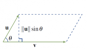
This expression for  makes no reference to a coordinate system and, moreover, it has a nice geometrical interpretation. The parallelogram determined by the vectors and has base length and altitude
  . Hence the area of the parallelogram formed by and is

Theorem 4.3.4
If and are two nonzero vectors and is the angle between and , then:
-
 the area of the parallelogram determined by and .
 - and are parallel if and only if
 .
.
Proof of 2:
By (1), if and only if the area of the parallelogram is zero. The area vanishes if and only if and have the same or opposite direction—that is, if and only if they are parallel.
Example 4.3.1
Find the area of the triangle with vertices  ,
,  , and
, and  .
.
Solution:
We have
![\vec{RP} = \left[ \begin{array}{r} 1\\ 1\\ -1 \end{array} \right]](https://ecampusontario.pressbooks.pub/app/uploads/quicklatex/quicklatex.com-8e0f99a9ac49165517e8788da7002a04_l3.png "Rendered by QuickLaTeX.com") and
and ![\vec{RQ} = \left[ \begin{array}{r} 2\\ -1\\ 0 \end{array} \right]](https://ecampusontario.pressbooks.pub/app/uploads/quicklatex/quicklatex.com-85bba21038b87b1ab05a3b0fb228a137_l3.png "Rendered by QuickLaTeX.com") . The area of the triangle is half the area of the parallelogram formed by these vectors, and so equals
. The area of the triangle is half the area of the parallelogram formed by these vectors, and so equals  . We have
![\begin{equation*} \vec{RP} \times \vec{RQ} = \func{det}\left[ \begin{array}{rrr} \vect{i} & 1 & 2\\ \vect{j} & 1 & -1\\ \vect{k} & -1 & 0 \end{array} \right] = \left[ \begin{array}{r} -1\\ -2\\ -3 \end{array} \right] \end{equation*}](https://ecampusontario.pressbooks.pub/app/uploads/quicklatex/quicklatex.com-eb3aa9ea2f18cf128fd3f57759e13e88_l3.png "Rendered by QuickLaTeX.com")
so the area of the triangle is 
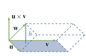
If three vectors , , and are given, they determine a “squashed” rectangular solid called a parallelepiped (Figure 4.3.2), and it is often useful to be able to find the volume of such a solid. The base of the solid is the parallelogram determined by and , so it has area  . The height of the solid is the length of the projection of on . Hence

Thus the volume of the parallelepiped is  . This proves
Theorem 4.3.5
The volume of the parallelepiped determined by three vectors , , and is given by  .
.
Example 4.3.2
Find the volume of the parallelepiped determined by the vectors
![\begin{equation*} \vec{w} = \left[ \begin{array}{r} 1\\ 2\\ -1 \end{array} \right], \vec{u} = \left[ \begin{array}{r} 1\\ 1\\ 0 \end{array} \right], \vec{v} = \left \begin{array}{r} -2\\ 0\\ 1 \end{array} \right] \end{equation*}](https://ecampusontario.pressbooks.pub/app/uploads/quicklatex/quicklatex.com-c1a3639375f2f032e95ae837e9db2907_l3.png "Rendered by QuickLaTeX.com")
Solution:
By Theorem 4.3.1, ![\vec{w} \cdot (\vec{u} \times \vec{v}) = \func{det}\left[ \begin{array}{rrr} 1 & 1 & -2\\ 2 & 1 & 0\\ -1 & 0 & 1 \end{array} \right] = -3](https://ecampusontario.pressbooks.pub/app/uploads/quicklatex/quicklatex.com-dadaf0056ccc8ff2bd530976887f32ad_l3.png "Rendered by QuickLaTeX.com") .
.
Hence the volume is  by Theorem 4.3.5.
We can now give an intrinsic description of the cross product .
Right-hand Rule
If the vector is grasped in the right hand and the fingers curl around from to through the angle , the thumb points in the direction for 
To indicate why this is true, introduce coordinates in as follows: Let and have a common tail , choose the origin at , choose the axis so that points in the positive direction, and then choose the axis so that is in the – plane and the positive axis is on the same side of the axis as . Then, in this system, and have component form
![\vec{u} = \left[ \begin{array}{r} a\\ 0\\ 0 \end{array} \right]](https://ecampusontario.pressbooks.pub/app/uploads/quicklatex/quicklatex.com-8ec49bb62b33a46db460e74dd3641a3e_l3.png "Rendered by QuickLaTeX.com") and
and ![\vec{v} = \left[ \begin{array}{r} b\\ c\\ 0 \end{array} \right]](https://ecampusontario.pressbooks.pub/app/uploads/quicklatex/quicklatex.com-3efc17fe8f791104d26f5254e5220c2f_l3.png "Rendered by QuickLaTeX.com")
where and  . Can you draw a graph based on the description here?
The right-hand rule asserts that should point in the positive direction. But our definition of gives
![\begin{equation*} \vec{u} \times \vec{v} = \func{det}\left[ \begin{array}{rrr} \vect{i} & a & b\\ \vect{j} & 0 & c\\ \vect{k} & 0 & 0 \end{array} \right] = \left[ \begin{array}{c} 0\\ 0\\ ac \end{array} \right] = (ac)\vect{k} \end{equation*}](https://ecampusontario.pressbooks.pub/app/uploads/quicklatex/quicklatex.com-42229c22e002c59e3837ddce0fc126dd_l3.png "Rendered by QuickLaTeX.com")
and  has the positive direction because
  .
.
