Living Systems Lab Appendices
Overview
| Appendix | Description and Link |
|---|---|
| A | Microsoft Excel |
| B | Image J - Adding a scale bar - Calibrating measurement tools - Making linear measurements - Measuring area |
| C | Preparing Chemical Solutions - w/v% - v/v% - mol/l - g/l - Diluting and dilution factors |
| D | Video Editing |
| E | Microscopes - Axio Lab.A1 Compound - Axio Lab.A1 Compound, Kohler - Primostar Compound - Primostar Compound, Kohler - Primostar 3 Compound - Primostar 3 Compound, Kohler - Stemi 305 Stereoscope |
| F | Zen Software - Overview of Zen software and interface - Obtaining a live image - Optimizing the live image - Image capture and exporting - Video capture, editing and exporting - Software and microscope shutdown |
| G | Virtual Microscope |
Appendix A: Microsoft Excel
LSL Video Appendix - Microsoft Excel
Download the Excel file containing the UN data set that was used in the video so you can follow along.
Other helpful Excel resources:
How to add, change, or remove error bars in a chart
Relative, absolute and mixed cell references

ImageJ is free software that can be used to display, edit, and analyze images. For example, if you captured an image of a cell, you could open this image in ImageJ and measure the diameter of the cell or add a scale bar to the image. There are many tutorial documents and demonstration videos on YouTube if you need further assistance. Look at this link for additional ImageJ documentation and resources.
Adding a scale bar, calibrating the measurement tools, and taking linear measurements with ImageJ
LSL Video - ImageJ Part 1
This video demonstrates how to add a scale bar, calibrate the measuring tools, and take linear measurements using ImageJ. These directions are also explained in the steps and images below.
The directions below are modified from ImageJ set scale. (n.d.). Retrieved January 8, 2019, from http://microscopy.berkeley.edu/courses/dib/sections/04IPIII/IJsetscale.html
Calibrating the Measuring Tools and Adding a Scale Bar
Suppose you wish to gather measurements from an image using real values (µm, miles, etc.). The process involves calibrating a single image against known values, then applying that calibrated image to your unknown image. This assumes, of course, that both images are the same magnification. Here's an example.
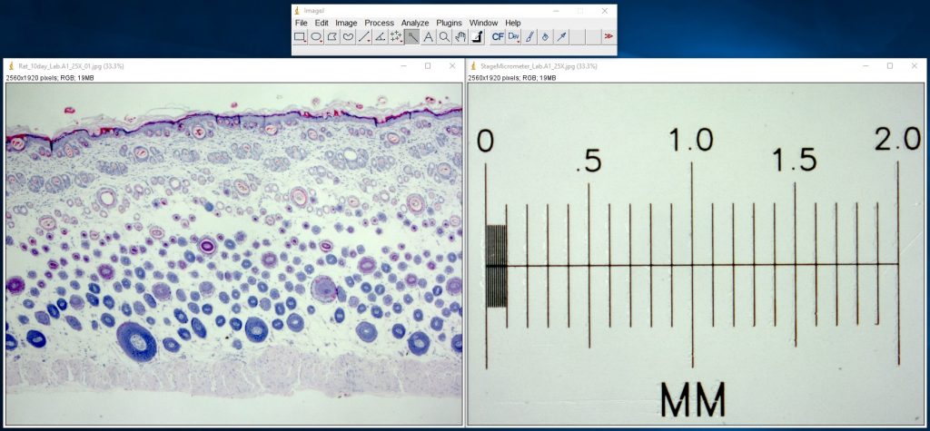
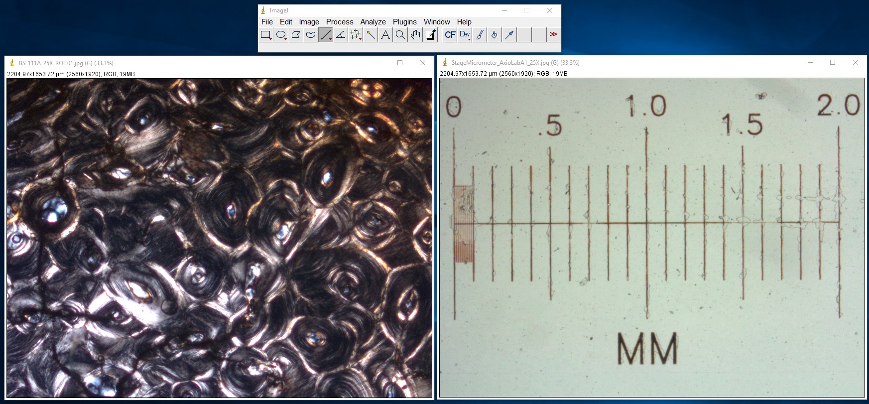
ImageJ Figure 1: Open your original image as well as a calibrated image. Here you see an image of a cross section of skin from a rat (left) and a microscope stage micrometer (right) . The stage micrometer is 2 mm (2000 μm) long. The smallest markings on the left (between 0 and 0.1 mm) are spaced 0.01 mm (10 μm) apart.
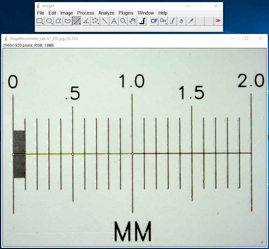
ImageJ Figure 2: Use the Line Selection tool to draw a selection line of a known length. Here we've drawn a 1000 µm line (the yellow line in the image)
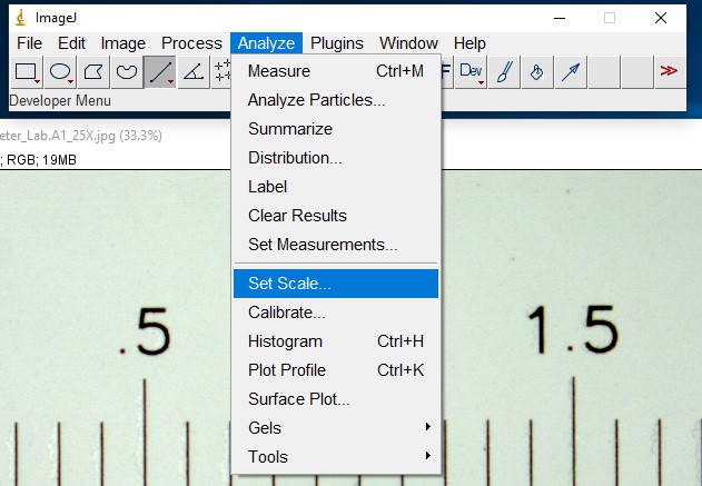
ImageJ Figure 3: With the selection line present, select "Set Scale" from the Analyze menu
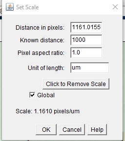
ImageJ Figure 4: This brings up the 'set scale' dialog box. Fill in the known distance (1000 µm) and Unit of Length (µm) fields . Check the "Global" checkbox. This spatial calibration will be applied to all open image windows. Click OK. Note: The known distance and unit of length will vary depending on how long you make the line on the image of the stage micrometer, and what units you want to use.
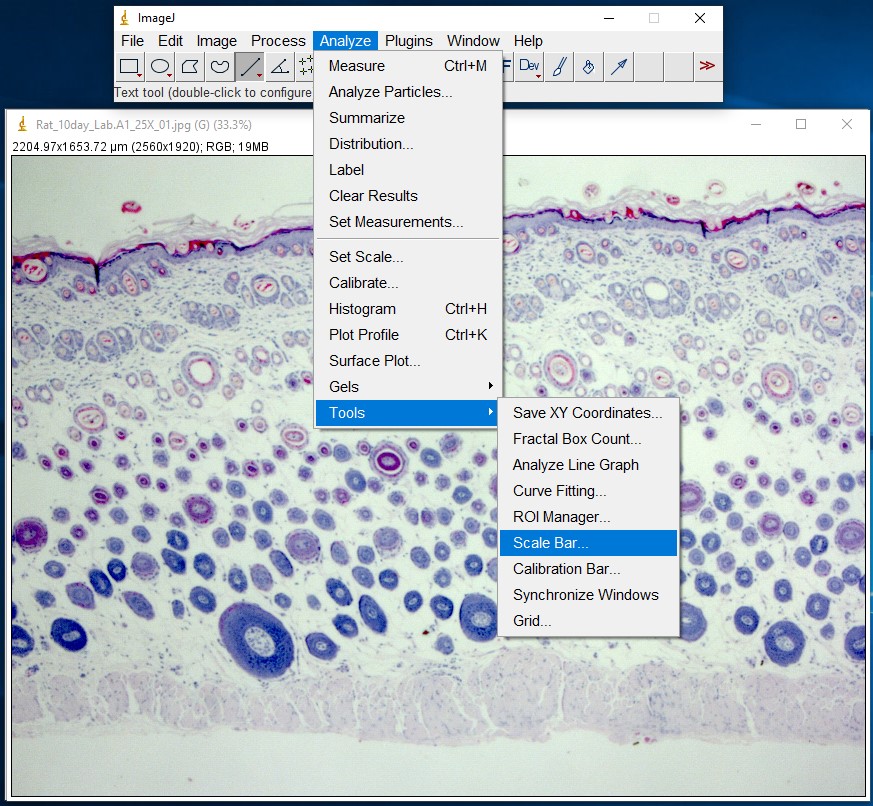
ImageJ Figure 5: You can add a scale bar to your image by choosing Analyze > Tools > Scale Bar.
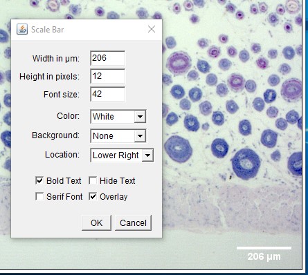
ImageJ Figure 6: This brings up the 'scale bar' dialog box. Make changes in the different fields (e.g. width, colour, location) to modify the appearance of the scale bar.
Taking a Linear Measurement
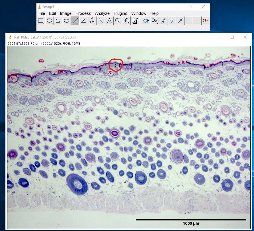
ImageJ Figure 7: Use the Line Selection tool to draw a selection line along the structure you wish to measure. In this example, the length of the epidermis is being measured in a cross section of skin obtained from a rat. The selection line (appearing in yellow in ImageJ) has been outlined in red so you can see it more easily. If needed, you can zoom in on the image (in ImageJ) to take a more accurate measurement. Use the magnifying glass, the '+' or "-" keys on the keyboard, or hold down control and use the scroll ball on the mouse to change the level of zoom.
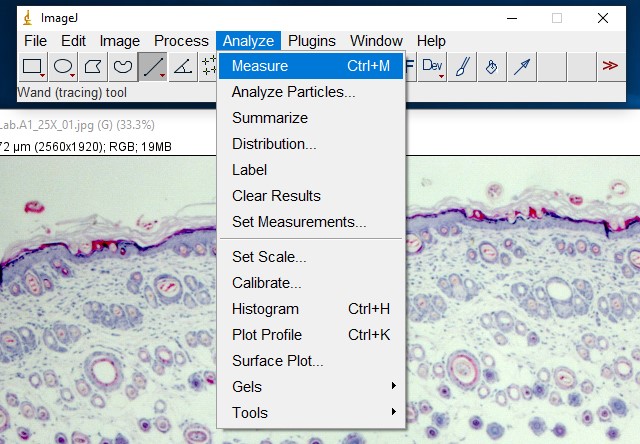
ImageJ Figure 8: Select Analyze > Measure to obtain the length of the selection line.
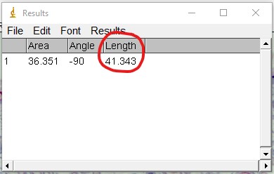
ImageJ Figure 9: This brings up the 'results' dialog box. The length of the yellow line is displayed. It is outlined in red so you can see it more easily. The units will depend on which units you applied when calibrating the scale bar. In this case, it is 41.343 µm.
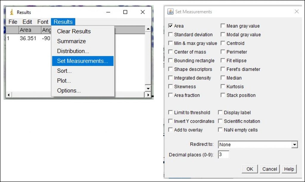
ImageJ Figure 10:You can toggle the display of different measurements (e.g. area, perimeter etc.) that show up in the results box by choosing Results > Set Measurement. This will open the 'set measurement' dialog box, where you can and enable or disable the measurements you would like displayed.
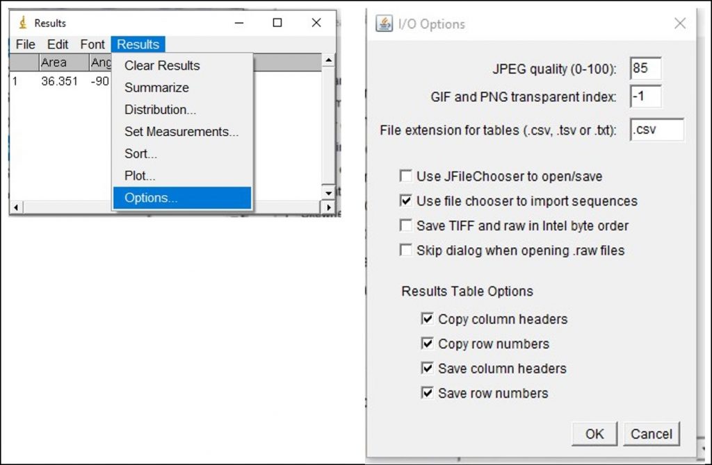
ImageJ Figure 11: You will likely need to take many measurements and analyze the data in Excel. To copy all of the values from the ImageJ results with the column headings, go to Results > Options. This will open the 'I/O Options' dialog box. Ensure ‘copy column headers’ is enabled. This will allow you to copy all of the data from the results window, including the column headings. Go back to the results window and select all the data (Edit > Select All or 'Control + A'). Next, copy all the data (Edit > Copy or 'Control + C'). Open up an Excel file and paste the data into the spreadsheet by selecting an empty cell and pressing 'Control +V'. The data values with column headings should appear. You can now analyze the data in Excel.
Measuring Area With ImageJ
LSL Video - ImageJ Part 2
This video reviews how to calibrate the measuring tools and demonstrates how to measure area (e.g. in mm2) using ImageJ. These directions are also explained in the steps below.
ImageJ Figure 12: Open your image as well as a calibrated image. Here you see an image of a cross section of bone (left) and a microscope stage micrometer (right). Calibrate the scale as described above (ImageJ figures 1-4).
ImageJ Figure 13: Use either the freehand or the polygon selection tool to trace the outline of the structure of which you wish to measure the area. In the example below, a single osteon has been outlined. The selection line will appear yellow in ImageJ. Next, select Analyze > Measure
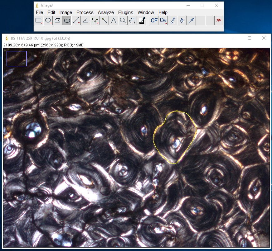
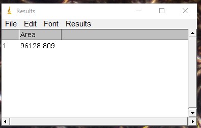
ImageJ Figure 14: This brings up the 'results' dialog box. The area of the object you traced is displayed. The units will depend on which units you applied when calibrating the scale bar. In this case, it is 96128 µm2.
Are your ImageJ values realistic?
After taking a few measurements with ImageJ, step back and look at the data. Are the numbers sensible?
For example, let's estimate the area of a hypothetical osteon and compare it to the area of the osteon we measured in imageJ above.
Recall the diameter of an osteon is around 0.2 mm/200 µm. Let's assume this hypothetical osteon was a perfect circle. The area of a circle is:
Area = πr2
Therefore, the area of a hypothetical osteon that is a circle with a diameter of 0.2 mm is:
Area = (3.14)(0.1)2
Area = 0.0314 mm2 (or 31400 µm2)
The area of the osteon we measured is 96128 µm2. This value seems realistic - its about 3X bigger, and not say, 1000X times bigger (which may indicate an issue with the calibration).
While ImageJ can be a powerful tool to help you analyze data, it is only as good as the critical thinking of the scientist using it.
Appendix C: Preparing Chemical Solutions
The concentration of chemical solutions can be represented in different ways as described below.
Note the following terms:
Solute: substance that dissolves [e.g. solid sodium chloride, NaCl(s)]
Solvent: substance that enables solute to dissolve [e.g. liquid water, H2O(l)]
Solution: mixture of solute dissolved in solvent [e.g. sodium chloride dissolved in water, NaCl(aq)]
Formula: Percentage by weight (w/v%) = [latex]\frac{mass\;of\;solute\;(g)}{Total\;volume\;of\;solution\;(ml)}[/latex] x 100
Example: Prepare 150 ml of a 10% sucrose solution
How much sucrose (g) do you need?
Let mass of sucrose = x
10% = [latex]\frac{x\;(g)}{150\;(ml)}[/latex] x 100
10 = [latex]\frac{100x}{150}[/latex]
100x = 1500
x = 15
Directions: Weigh out 15 grams of sucrose and dissolve in approximately 115 ml of H20. Once fully dissolved, bring the final volume of the solution to 150 ml.
Note: Total volume of solution = volume from solvent (e.g. water) plus the volume from solute (e.g. sucrose). Using the example above, you do not want to add 15 grams to 150 ml, as the sucrose itself will cause the final volume to be > 150 ml.
Formula: Percentage by volume (v/v %) = [latex]\frac{Volume\;of\;solute\;(ml)}{Total\;volume\;of\;solution\;(ml)}[/latex] x 100
Example: Prepare 250 ml of a 30% propylene glycol solution (starting with a stock solution of 100% propylene glycol)
How much propylene glycol (ml) do you need?
Let ml of propylene glycol = x
30% = [latex]\frac{x\;(ml)}{250\;(ml)}[/latex] x 100
30 = [latex]\frac{100x}{250}[/latex]
100x = 7500
x = 75
Directions: Measure out 75 ml of propylene glycol and add to just under 175 ml of H20 (250 – 75), then bring the final volume to 250 ml.
Note: In the lab, you might have added 100 μl of propylene glycol to a final total volume of 1000 μl (100 μl of propylene glycol, 850 μl of H20, and 50 μl of dye) to give you a 10% solution of propylene glycol with food colouring. In this case, the solvent was: H20 + food colouring.
Prepare solutions of a certain concentration from a solid solute:
Molarity (M or mol/l)
Formula: [latex]C=\frac{n}{V}[/latex]
Where:
C = concentration of solution in mol L-1 (mol/l or M),
n = moles of substance being dissolved (moles of solute),
V = volume of solution in litres (l)
Example: Prepare 1 L of a 1M solution of sucrose
Molarity is the number of moles of a chemical/solute in 1000 ml of H20 i.e. moles per litre
If you add one mole of sucrose to H20 and bring the final volume of 1000 ml, you would have a 1M or 1 moles/L solution of sucrose.
But, wait, how do you weigh out 1 mole of sucrose??
You need the molecular weight of the solute to prepare such a solution.
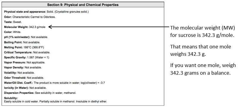
The molecular weight (MW) of sucrose can be found on the bottle, in the SDS or from the manufacturer.
Here is a portion of the SDS for sucrose:
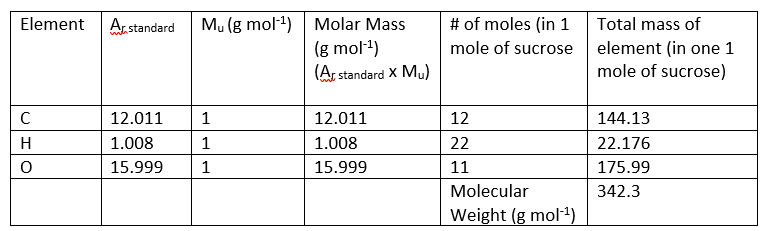
Note the standard atomic weight (or relative atomic mass) is a ratio, and hence dimensionless, and the molar mass constant = 1 g mol-1. Therefore, the molar mass of each element (in g mol-1) will be the same value as the standard atomic weight, however, the molar mass will have units (g mol-1)
The # of atoms of each element in the compound can be obtained from the molecular formula. For example, 1 compound of sucrose contains 12 atoms of carbon (C), 22 atoms of hydrogen (H) and 11 atoms of oxygen (O). This may also be expressed as 1 mole of sucrose containing 12 moles of carbon (C), 22 moles of hydrogen (H) and 11 moles of oxygen (O).
Using this information, we can calculate the molecular weight of sucrose:
Example: Prepare 1 L of a 1M solution of sucrose (continued)
So, weigh 342.3 g of sucrose and dissolve in ~750 ml H20. Then bring the final volume to 1000 ml (1 L).
Note: this is different from adding the sucrose into 1000 ml of water. Since the sucrose itself takes up volume in the solution, you need to initially dissolve the sucrose in a smaller volume of water, and then add additional water until your final volume is 1000 ml.
Maybe you don’t need 1000 ml of this solution. If you want to make only 50 ml, you will need to modify accordingly:
[latex]\frac{342.3\;g}{1000\;ml}\;=\;\frac{x\;g}{50\;ml}[/latex]
Solving for x will give you 17.115 g.
Therefore, you will weigh out 17.12 g of sucrose and dissolve it in a final volume of 50 ml of H20. For example, you would add 17.12 g of sucrose into 30 ml of H20. Once the sucrose dissolved, you would bring the final volume of the solution to 50 ml.
Prepare solutions of a certain concentration from a solid solute:
g/l
The concentration of the solute in this solution would be expressed as g/l (using the example units given above).
For example, suppose you wanted to make a solution of silver (Ag) at a concentration of 1 g l-1. You would need to dissolve 1 g of silver in water and bring the final volume to 1 litre. But…you can’t dissolve solid silver in water. How would you prepare this solution?
You have to dissolve a silver-containing salt, where silver will dissociate once added to water.
For example, silver nitrate: AgNO3.
But…if you add 1 g of silver nitrate into the water, you won’t have 1 g of silver. You will have a mixture of silver (Ag) and Nitrate (NO3).
How much silver nitrate do you need to add to water to have 1 g of silver?
Recall the molecular formula tells us how many moles of each element are in the compound. So 1 mole of AgNO3 salt contains 1 mole of silver, 1 mole of nitrogen and 3 moles of oxygen.
We can multiply the molar mass of each element by the number of moles present in the compound:
Ag = 107.87 g mol-1 x 1 mole = 107.87 g of silver
N = 14.007 g mol-1 x 1 mole = 14.007 g of nitrogen
O = 15.999 g mol-1 x 3 moles = 47.997 g of oxygen
Molecular Weight of AgNO3 = 107.87 + 14.007 + 47.997 = 169.87 g mol-1
Therefore, 1 mole of AgNO3 weighs 169.87 g and contains 107.87 g of silver (Ag).
So, how many grams of AgNO3 will contain 1 g of silver?
[latex]\frac{169.87\;g\;of\;AgNO_3}{x\;g\;of\;AgNO_3}\;=\;\frac{107.87\;g\;of\;Ag}{1\;g\;of\;Ag}[/latex]
169.87 = 107.87x
x = 1.57
Therefore, 1.57 g of AgNO3 salt will contain 1 g of silver. So we would dissolve 1.57 g of AgNO3 in water, and bring the final volume to 1 liter to make a solution that contains 1 g Ag l-1.
Diluting and Dilution Factors
Dilution Factors
Suppose you prepared 1000 ml of a stock solution of atropine at a concentration of 10-3 mol l-1 (=0.001 mol l-1 = 1 mmol l-1 = 1000 µmol l-1).
If you were asked to dilute the stock solution 10X (or 10-fold) and have a final volume of 100 ml, how would you do this? Assume you are diluting the stock with saline.
The dilution factor (DF) can be calculated as:
[latex]DF=\frac{Final\;Volume}{Aliquot\;Volume}[/latex]
[latex]Final\;volume\; =\; aliquot\; volume\; +\; diluent\; volume[/latex]
In our example:
Final volume = 100 ml. This could be a different volume, depending on how much diluted solution you need.
Aliquot volume = refers to the volume of atropine stock
Diluent volume = refers to the volume of saline (what you are using to dilute the stock atropine)
Important: You must keep your units the same (e.g. ml)
Therefore:
[latex]DF=\frac{Aliquot\;Volume\;+\;Diluent\;Volume}{Aliquot\;Volume}[/latex]
Using the example above, if we wish to dilute the atropine stock 10X (10-fold), and have a final volume of 100 ml:
[latex]DF=\frac{Final\;Volume}{Aliquot\;Volume}[/latex]
[latex]10=\frac{100}{Aliquot\;Volume}[/latex]
[latex]100\;=\;10\;*\;aliquot\;volume[/latex]
[latex]Aliquot\;Volume\;=\frac{100}{10}[/latex]
[latex]Aliquot\;Volume\;=10\;ml[/latex]
The aliquot volume (10 ml) is the amount of atropine stock we need. To figure out how much diluent (= saline) we need, recall that:
[latex]Final\;Volume\;=Aliquot\;Volume\;+\;Diluent\;Volume[/latex]
[latex]100\;=\;10\;+\;Diluent\;Volume[/latex]
[latex]Diluent\;Volume\;=\;100\;-\;10[/latex]
[latex]Diluent\;Volume\;=\;90[/latex]
Therefore, 10 ml of atropine stock (aliquot volume) + 90 ml of saline (diluent volume) gives a final volume of 100 ml and a stock that was diluted 10X.
What would be the concentration of 10X diluted stock? It would be the concentration of the stock solution (0.001 mol l-1) divided by the DF (=10):
[latex]Concentration\;of\;diluted\;solution\;=\frac{Original\;concentration\;of\;stock}{Total\;Dilution\;Factor}[/latex]
[latex]Concentration\;of\;diluted\;solution\;=\frac{0.001}{10}[/latex]
[latex]Concentration\;of\;diluted\;solution\;=\;0.0001\;mol\;l\;^-\;^1\;(10\;^-\;^4\;mol\;l\;^-\;^1)[/latex]
If you dilute this 10-4 mol l-1 solution by 10X again, your total dilution (of the stock) is the product of all the dilution factors:
[latex]Total\;Dilution\;Factor\;=\;DF_1\;*\;DF_2[/latex]
[latex]Total\;Dilution\;Factor\;=\;10\;*\;10[/latex]
[latex]Total\;Dilution\;Factor\;=\;100[/latex]
This is a serial dilution - a series of solutions in which each subsequent solution is diluted 10X.
Note: If you had a solution where the concentration is expressed in some other units (e.g. %), the same methods apply. For example, if you had a solution of 95% ethanol (EtOH) and diluted it 10X, you would mix 10 ml of 95% EtOH + 90 ml of diluent, and the concentration would be 95%/10 = 9.5% EtOH.
Diluting
What if you were asked to prepare a specific volume and concentration from a stock solution?
For example, you prepare a stock solution of atropine at a concentration of 0.001 mol l-1 (= 1 mmol l-1 = 1000 µmol l-1)
You are asked to prepare 50 ml of 100 µmol l-1 atropine. You are told to dilute the stock using saline as the diluent.
A simple way to figure this out is to use the formula:
[latex]C_1\;V_1\;=\;C_2\;V_2[/latex]
C1 = the concentration of the stock atropine (=1000 µmol l-1)
V1 = the volume of the stock that is needed (e.g. in ml). This is unknown and we will solve for it.
C2 = the desired concentration of the atropine (=100 µmol l-1)
V2 = the final volume of the solution (e.g. in ml). This is the final volume you want (=50 ml) and is made up of the volume of the stock and the volume of the diluent (what you are using to dilute the stock).
In addition:
[latex]Final\;Volume\;=\;V_2\;=\;V_1\;+\;Diluent\;Volume[/latex]
[latex]Diluent\;Volume\;=\;V_2-V_1[/latex]
IMPORTANT: You must keep your units for C1 and C2 the same (in our example I chose µmol l-1) and the units for V1 and V2 the same (in our example I chose ml).
[latex]C_1\;V_1\;=\;C_2\;V_2[/latex]
1000 µmol L-1 x V1 = 100 µmol L-1 x 50 ml
[latex]V_1\;=\;\frac{(100)(50)}{1000}[/latex]
[latex]V_1\;=\;5\;ml[/latex]
[latex]Diluent\;Volume\;=\;V_2-V_1[/latex]
[latex]Diluent\;Volume\;=\;50-5[/latex]
[latex]Diluent\;Volume\;=\;45\;ml[/latex]
Therefore, you would measure out 45 ml of diluent (saline) and add 5 ml of the atropine stock to the diluent to obtain 50 ml of atropine at a concentration of 100 µmol l-1
Diluting Multiple Stocks to Make Mixtures
You can use the C1V1 = C2V2 formula for mixtures as well.
For example, suppose you are setting up a reaction that requires 10% EtOH and 50 µmol l-1 of atropine.
Your EtOH stock is 95% and the atropine stock is 1000 µmol l-1. The final desired volume of the mixture is 100 ml.
It may help to visualize this mixture using a table first. We can look at each compound individually, but the final volume, V2, will be the same for both compounds, because they are going into the same solution.
It is also important to note that we still need to add a diluent to bring the final solution to the total desired volume.
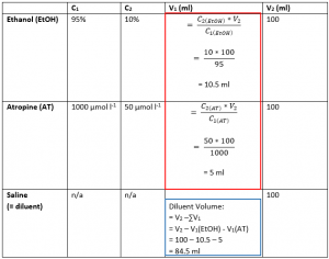
We start by filling in V1 for Ethanol and Atropine. This follows the standard C1V1 = C2V2 formula. The values for initial and final concentration for both Ethanol and Atropine were provided in the question, and the final volume of the solution was also given. These calculations are shown in the table above in the red box.
Next, having found the initial volumes for EtOH and AT, the volume of diluent (in this case saline), can be found by subtracting the volumes of the AT and EtOH solutions from the final volume. This calculation is shown in the table above in the blue box.
Therefore, you would measure out 84.5 ml of diluent (saline) and add 10.5 ml of the EtOH stock and 5 ml of the atropine stock to the diluent to obtain 100 ml of solution with a concentration of 10% EtOH and 50 µmol l-1 atropine.
This method works for mixtures of more than two compounds as well. Often, mixtures called mastermixes are created when an experiment needs several identical compounds in many reaction vessels, such as when amplifying DNA by PCR. For example, if you needed to fill 20 small tubes with a mixture of 5 compounds, it is much more efficient to make the mixture of several compounds first (5 pipette steps), then aliquot the mixture into the 20 small tubes (20 pipette steps). The alternative would be putting each of the 5 compounds into the 20 tubes one-by-one: a total of 100 pipette steps! Not only does preparing a larger mastermix before filling the tubes save time, it also reduces the chances of error. The ratio of the compounds in the mastermix is fixed, and therefore every tube will have the same ratio, which makes your experiment more robust.
Appendix D: Video Editing
QuickTime
Download QuickTime (you may need to download a different version depending on your specific operating system)
Windows: https://support.apple.com/kb/DL837?locale=en_US
Mac: https://support.apple.com/kb/dl923?locale=en_US
- Open your video file in QuickTime (File > Open File)
- A new window will open up and play your video.
- To capture still images of individual frames as the video plays, pause the video, then select Edit > Copy. Record the time.
- Paste this image into any image editing software (e.g. PowerPoint, Adobe, ImageJ)
- Within the image editing software, you can edit the image (e.g. crop, put multiple images together, add a graphic such as the time etc.)
iMovie (Mac OS only)
- Open iMovie.
- Create a "new movie” (⌘N)
- Import your movie using the toolbar (File > Import media or ⌘I), or drag it into iMovie.
- Your clip will appear in the top left part of your screen, the browser. Drag it down to the bottom, where it says “Drag and drop video clips and photos from the browser above to start creating your movie.” Here you can see the timestamp of each frame you move your cursor to along the video clip.
- When you have selected the frame you want to save, click the share icon at the top right of the screen, and save it as an image. You can repeat this for multiple frames.
- You can also add text (e.g. the time into the video clip that the still frame was taken from) to the image by clicking on the tab that says “Titles"
VLC Player
Download VLC media player (you may need to download a different version depending on your specific operating system)
Windows: https://www.videolan.org/vlc/download-windows.html
Mac: https://www.videolan.org/vlc/download-macosx.html
- Open your movie.
- Play your movie and pause on the frame you wish to capture. Or, select playback > jump to specific time (control + T) and enter the time you want to jump to.
- Select video > take snapshot
- An image of that frame will be saved as a .png on your computer in your ‘pictures’ folder.
- Paste this image into any image editing software (e.g. PowerPoint, Adobe, ImageJ)
- Within the image editing software, you can edit the image (e.g. crop, put multiple images together, add a graphic such as the time etc.)
Appendix E: Microscopes in the Living Systems Lab
Zeiss AxioLab.A1 Compound Microscope
Zeiss AxioLab.A1 - Kohler Illumination
Zeiss Primostar Compound Microscope
Zeiss Primostar - Kohler Illumination
Zeiss Primostar 3 Compound Microscope
Zeiss Primostar 3 - Kohler Illumination
Zeiss Stemi305 Stereomicroscope
Appendix F: Zen Software
Part 1: Overview of Zen software and interface
Note: The numbers in parentheses below correspond to the yellow numbers in the figures provided throughout.
- Turn on the computer and log into the guest account.
- Check that the USB camera cable is connected to the computer and wait for the light on the camera (blue square prism located on top of the microscope) to turn green. Once the light turns green, open the ZEN software from the shortcut on the desktop.
- Place a slide on the mechanical stage. Follow the directions in Appendix 1A/1B to bring the slide into focus with transmitted light for brightfield Köhler illumination. Adjust the microscope to correct for ametropia and the interpupillary distance of your eyes.
- Look through the eye pieces and adjust the light intensity of the microscope and aperture diaphragm until you can see a clear image of the specimen with appropriate contrast.
- Do not attempt to capture images until you can clearly see the specimen through the microscope optics.
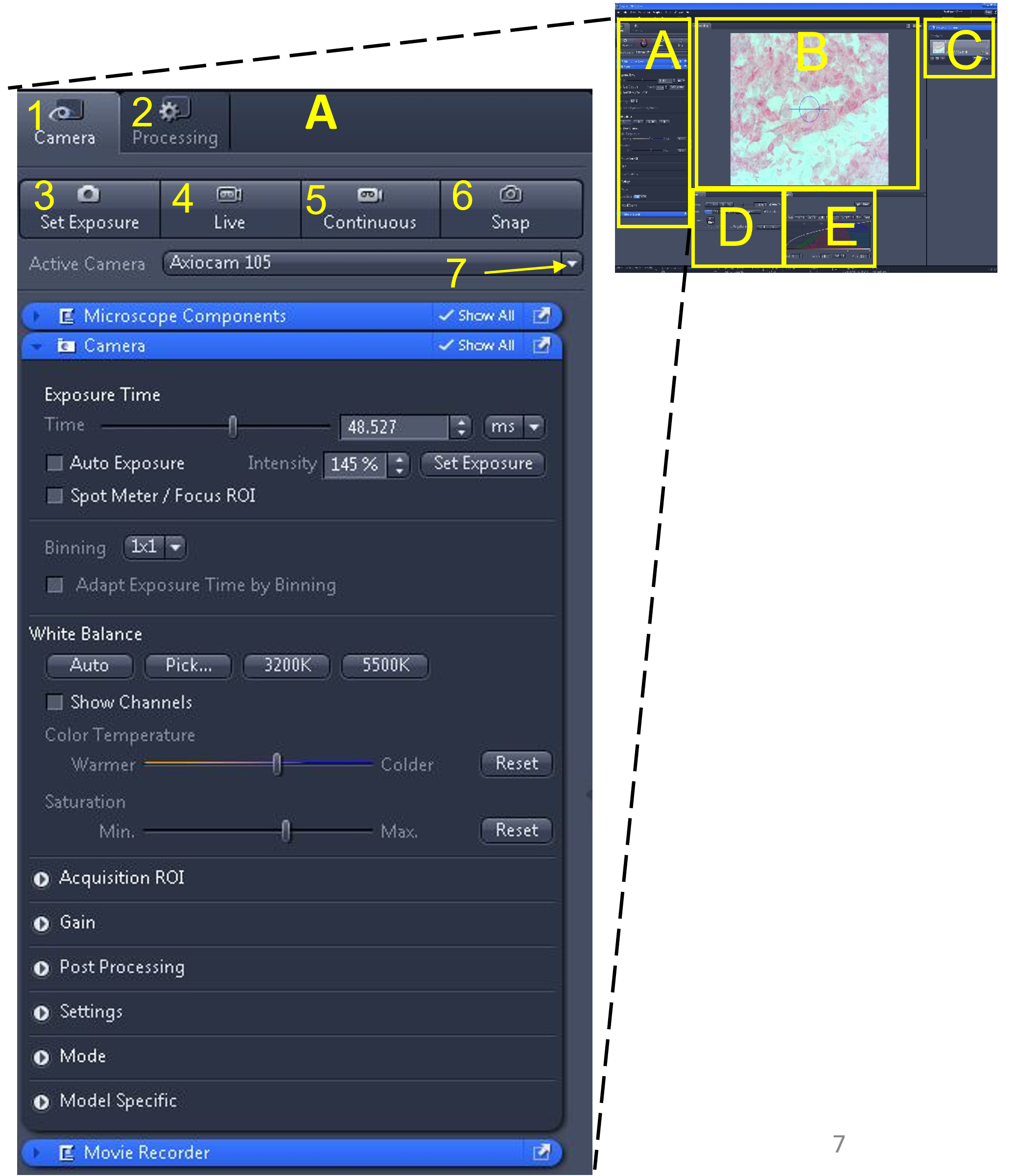
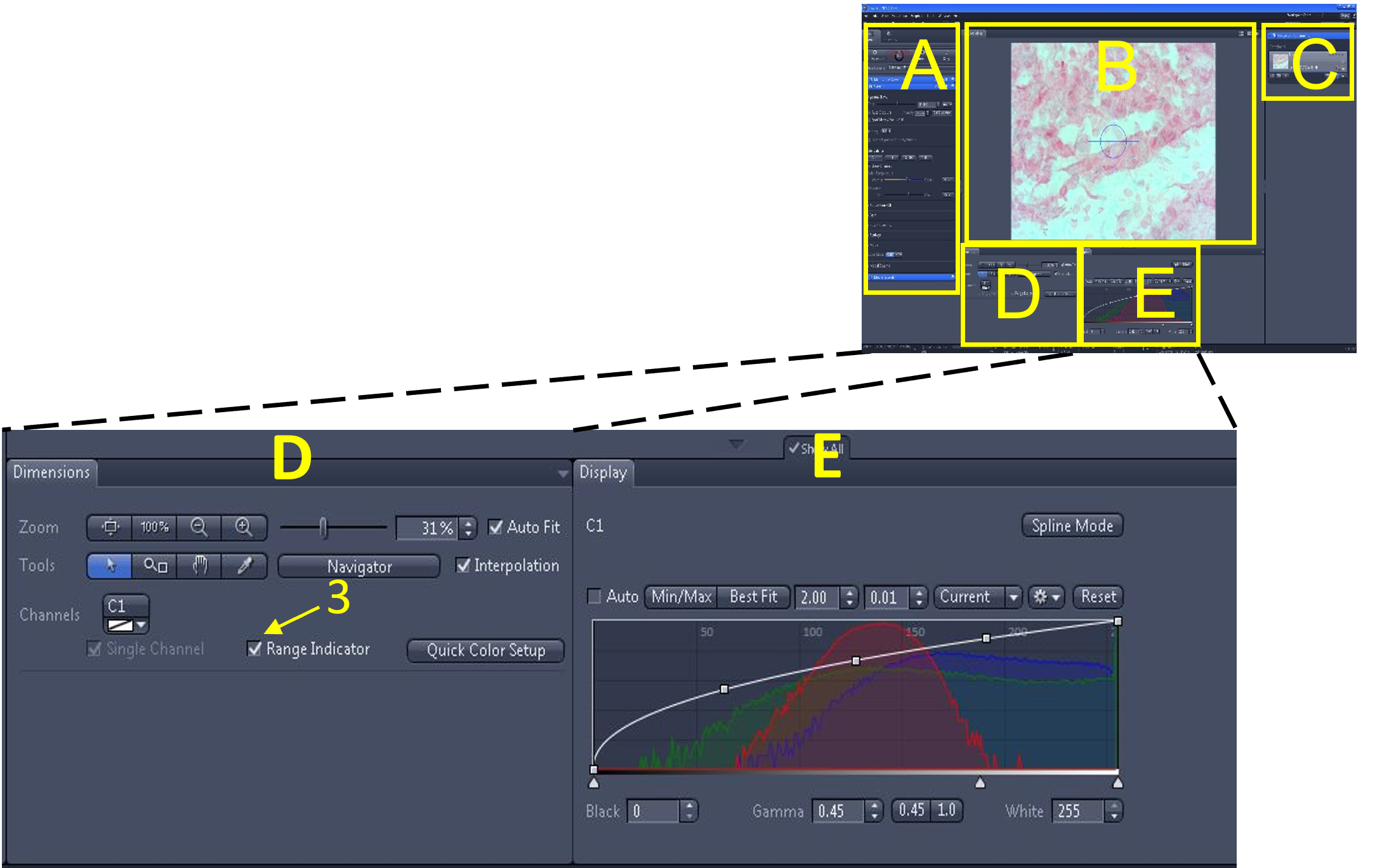
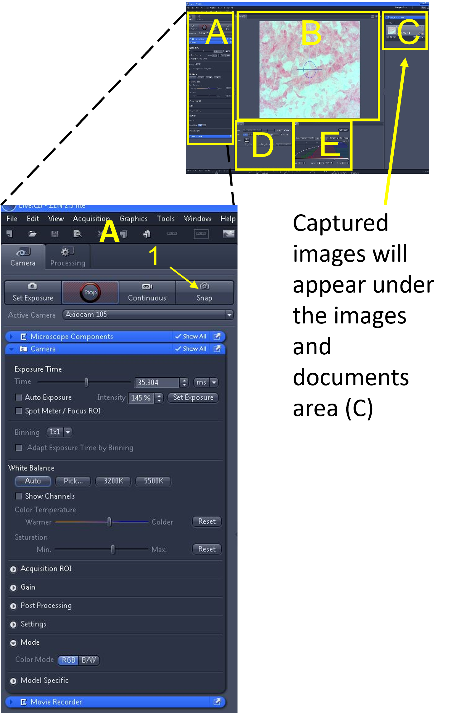
Zen Figure 1: Overview of Zen software and interface.
Part 2: Obtaining a live image
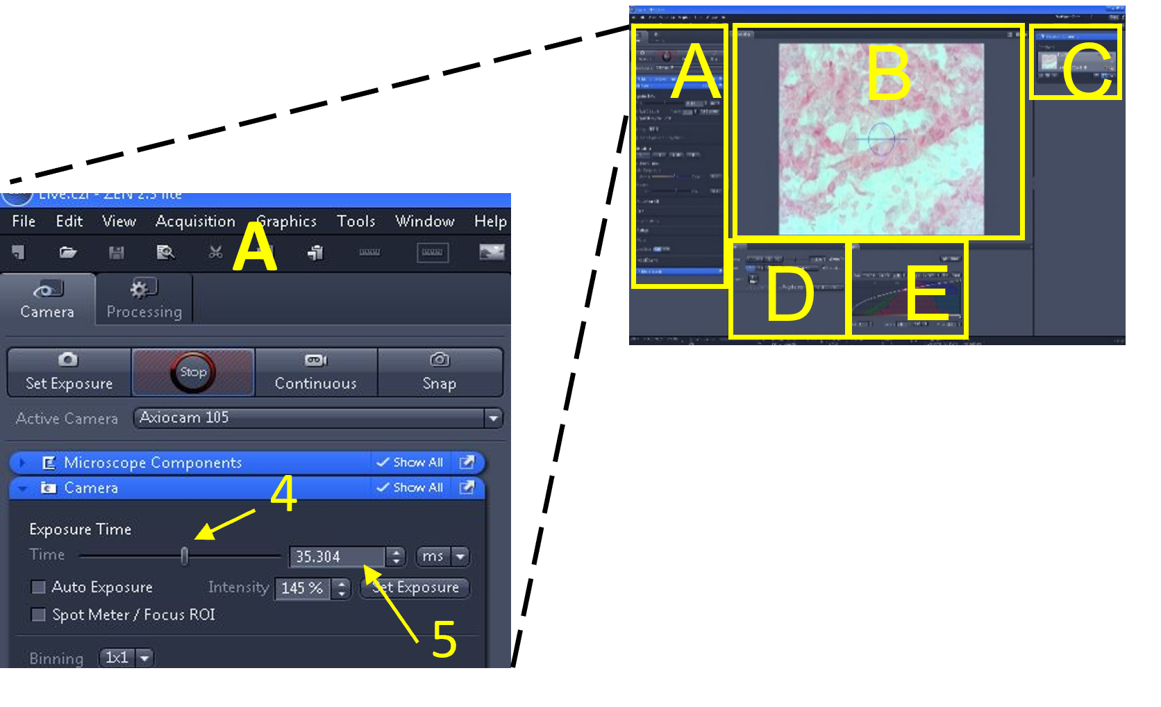
- Located at the top left of the software interface is the main tool area (A). Within this area are two menus: Camera (1) and Processing (2). The camera menu is used for viewing slides and capturing images or videos. The processing menu is used to edit images (among other things).
- Select the camera menu (1). Below the camera menu are four buttons: set exposure (3), live (4), continuous (5), and snap (6).
- Below these buttons is an 'active camera' drop down menu (7). Make sure the Axiocam 105 is selected from the drop down menu. If there are multiple cameras connected to the computer, you will need to see which one corresponds to the microscope you are currently using by trial and error. If you do not see any cameras listed in the drop down menu, exit the software, make sure the green light is illuminated on the camera, and restart the software.
- Select live (4).
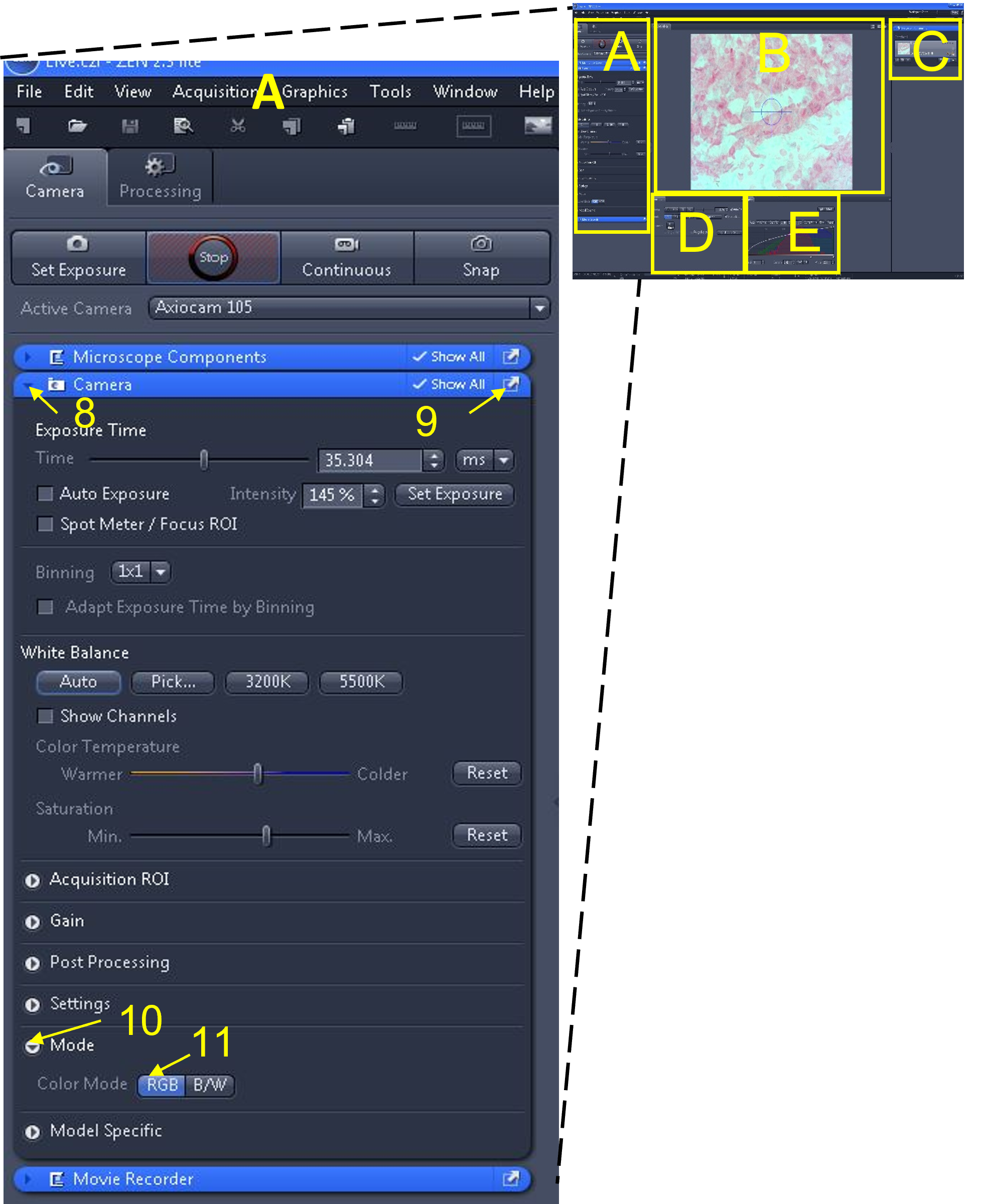
Zen Figure 2: Obtaining a live image #1. - A live image of the slide will appear in the middle display window (B). Do not worry if the image appears too bright or dark - we will fix this shortly.
- You may need to make very minor adjustments with the fine focus knob on the microscope to bring the image into focus in the software (the plane of focus for the camera and objective is not always identical).
- Make sure the camera is in colour (RGB) mode. To do this, open the camera tab submenu (8), by clicking on the triangle to the left of the word 'camera' in the blue bar.
- Enable the 'show all' box (9) in this camera tab submenu - this will make additional options appear.
- Click the mode button (10) and change to RGB (11), which is the colour camera mode. Note: B/W is for black and white mode.
Part 3: Optimizing the live image
Remember: Do not attempt to capture images unless you can clearly see the specimen through the microscope optics. Otherwise, you will never obtain a high quality image!
- If an image is overexposed, you can decrease the light intensity on the microscope and/or decrease the exposure time.
- If an image is underexposed, you can increase the light intensity on the microscope and/or increase the exposure time.
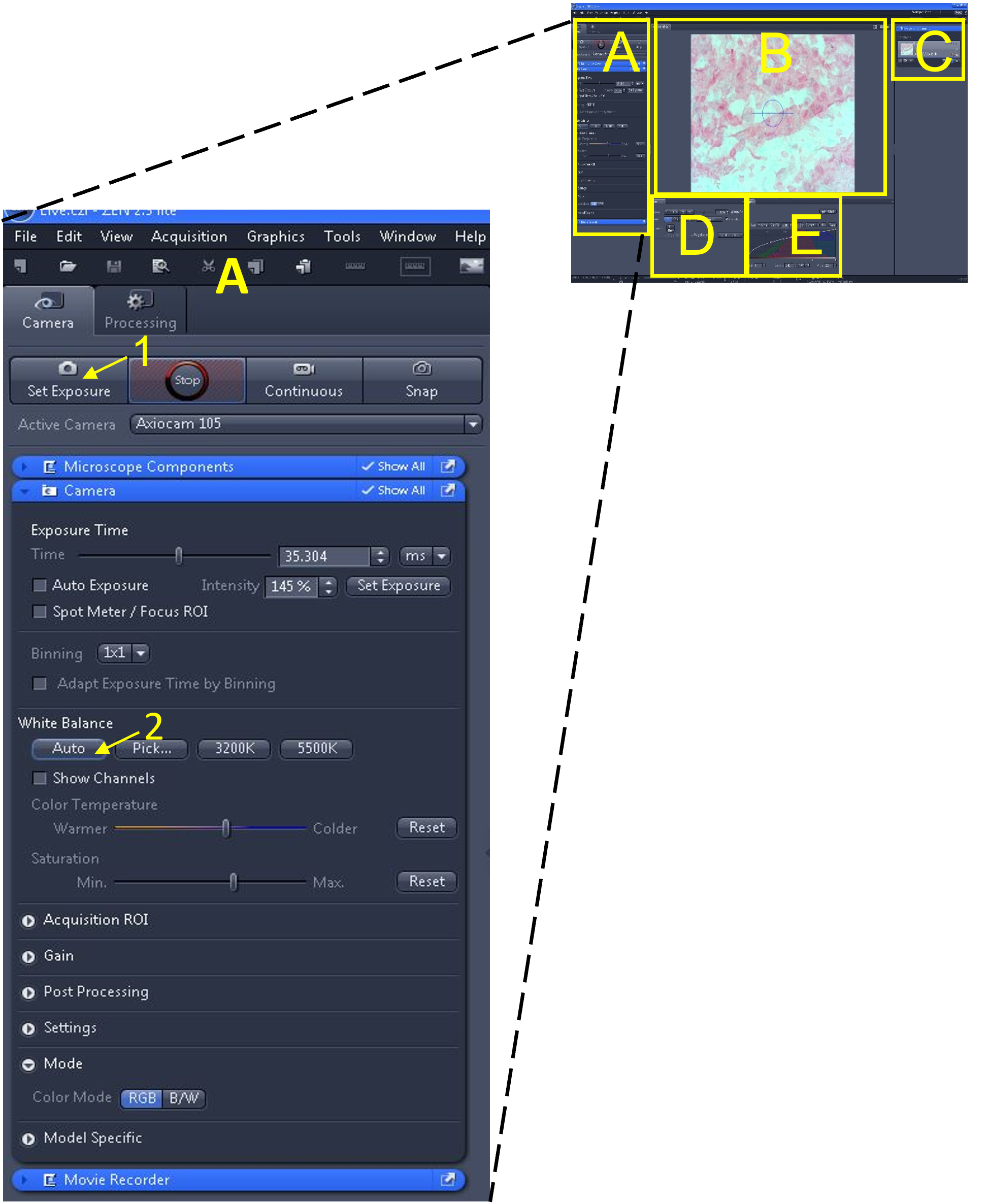
- In the main tool area (A) select the 'set exposure' button (1) - the software will automatically pick an exposure time based on the microscope's current light intensity.
- Adjust the white balance by clicking auto (2) under the white balance settings.
- Note: Next, we will use the 'range indicator' feature to located over- or under- exposed pixels and make minor adjustments to the exposure time to minimize them.
Zen Figure 4: Optimizing the live image #1
- Note: Next, we will use the 'range indicator' feature to located over- or under- exposed pixels and make minor adjustments to the exposure time to minimize them.
- In the image/video editing screen (D), enable the range indicator (3). Once enabled, pixels in the image display area (B) are highlighted red (too bright; overexposed) or blue (too dark; underexposed).
Zen Figure 5: Optimizing the live image #2. - In the main tool area (A), adjust the exposure time by either moving the exposure time slide bar (4) or changing the number in the exposure time box (5) until there are no (or very few) over- or under- exposed pixels being highlighted. Turn off the range indicator when done.
Zen Figure 6: Optimizing the live image #3. 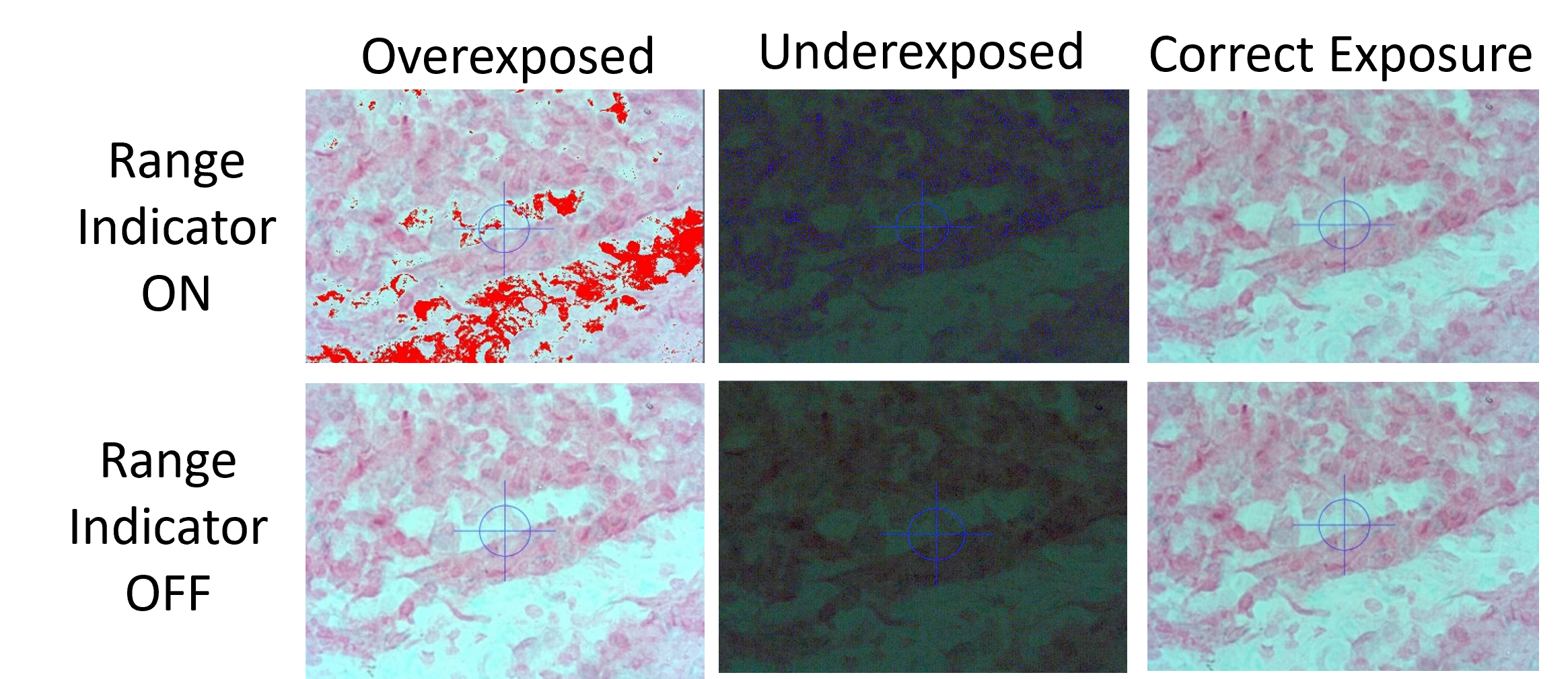
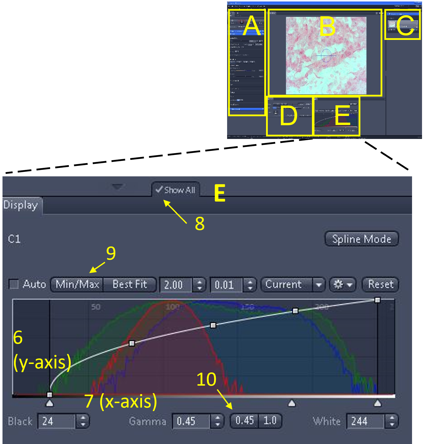
Zen Figure 7: Optimizing the live image #4. - The final part of optimizing the live image is to make adjustments via the histogram, which is located in the display settings area (E). For a colour camera, there are three overlaid histograms (red, green, and blue). The Y-axis (6) of the histogram indicates the number of pixels of each tone. The X-axis (7) indicates the pixel tone.
- Note: if you have the camera in B/W, there will only be one histogram. If you do not see all the different histogram options in the image shown here (e.g. min/max, best fit etc.), make sure the 'show all' button is enabled (8).
- The left side of the X-axis is pure black pixels. The right side of the X-axis is pure white pixels. In-between the pure black and pure white pixels are 256 graduations of coloured pixels (dark to light) for each of the channels (RGB).
- You can adjust the values under the histogram display curve including brightness (white), contrast (black) or gamma.
- Click min/max (9) and set gamma to 0.45 (10). Make minor adjustments from these values until you are satisfied with the image quality and there is sufficient contrast.
Zen Figure 8: Optimizing the live image #5.
Look at the difference optimizing the live image will have by comparing the four images (A-D).
Zen Figure 9: Image slider showing various captures of the same image to illustrate image optimization benefits. Hover over the image for the exposure information.
Summary of how to optimize the live image in Zen:
- Bring specimen into focus under the microscope. Use Köhler illumination and brightfield.
- Select 'set exposure' and adjust white balance with 'auto.'
- Use the range indicator to locate over or under exposed pixels. Make minor adjustments to the exposure time to minimize.
- Adjust the histogram. Use the min/max setting and set gamma to 0.45. Adjust further as needed.
Part 4: Capturing and saving images
Note: Complete parts 1-3 before trying to capture an image.
- Create a folder (e.g. L01_PodA) on the desktop to save your images on the computer. These images can then be uploaded to your Microsoft OneDrive folder on the web browser before you leave.
- Once you have an optimized live image of the specimen, select the 'snap' button (1) located in the main tool area (A). This will capture an image of the specimen.
- This captured image file will appear under the images and documents area (C), located on the right of the screen. If you can't see this area, the menu has been collapsed. To open it click on the 'show' triangle.
- You should see at least two files in the images and documents area - an image called live.czi and the image(s) you just snapped ('captured'). The name of the image(s) you captured will be called Snap-01.czi (or something similar).
- The extension .czi (= carl zeiss image) can only be opened with the Zen software. Save the .czi file in your group folder (in case you need to access the original file) and also save this image as a .jpg or .jpeg, which you can open using image analysis software (e.g. imageJ).
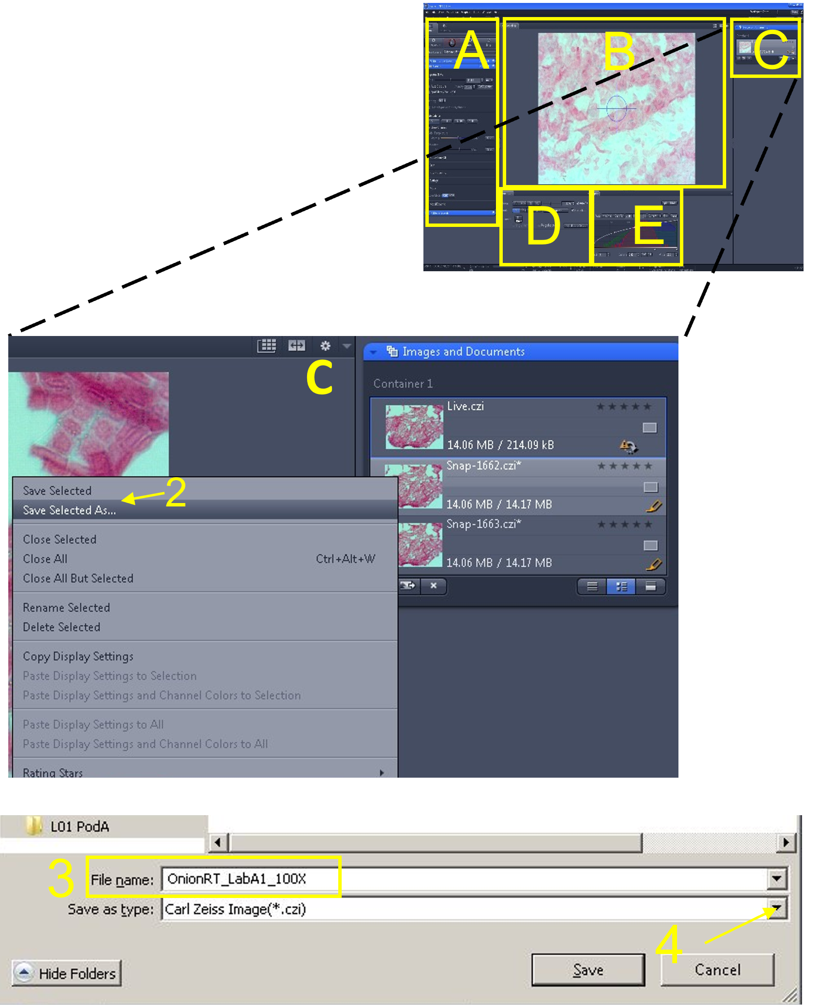
Zen Figure 9: Capturing and saving images #1. - First, save the image as a .czi file type in your desktop folder by clicking the image from the images and documents area (C), selecting 'Save Selected As' (2), selecting your folder as the destination, and saving the image in this folder. Include relevant information in the image file name (3) such as tissue type, microscope used and total magnification (e.g. OnionRT_AxioLabA1_100X). Repeat the step above, but before clicking save, click the 'save as type' drop down menu (4), and select .jpg or .jpeg as the extension.
- Once completed, open your group folder and make sure you can see two files - your .czi file and your .jpg file.
- Finish capturing images of your slides. Save all the images in the same folder.
- Once you are finished capturing images, lower the stage and remove the slide and return it to the slidebox.
- Upload only the .jpg images to your OneDrive folder.
Zen Figure 10: Capturing and saving images #2.
Part 5: Capturing, editing, and saving videos
Note: Complete parts 1-3 before trying to capture a video.
RECORDING THE VIDEO:
- Turn the camera to black and white mode (see part 2 above). Colour videos are very large flies and will fill the hard drive quickly.
- Turn up the light intensity on the microscope to its maximum brightness. If using the Stemi 305 stereoscope, use brightfield and the clear mirror, and adjust the inclination of the mirror for maximum brightness. This will ensure a low exposure time and thus maximize the frame capture rate (frames per second; FPS) when recording a video.
- Optimize the live image as previously described in part 3 of this appendix.
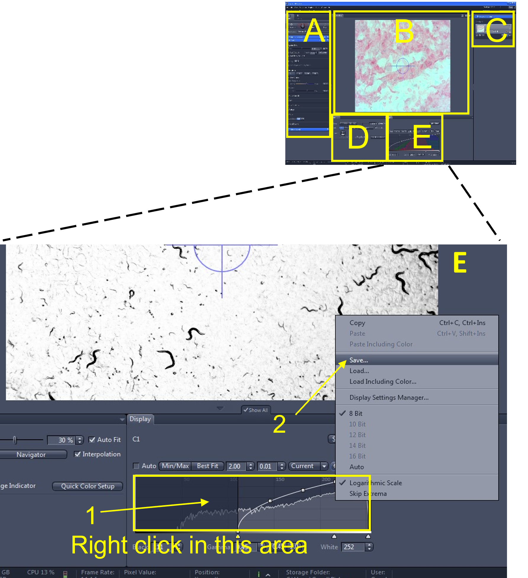
- In the display settings area (E), save these histogram settings by right clicking anywhere in the histogram display area (1) and selecting save (2). Use the default file directory and give the current histogram settings file a name (e.g. nematode_video_histogram).
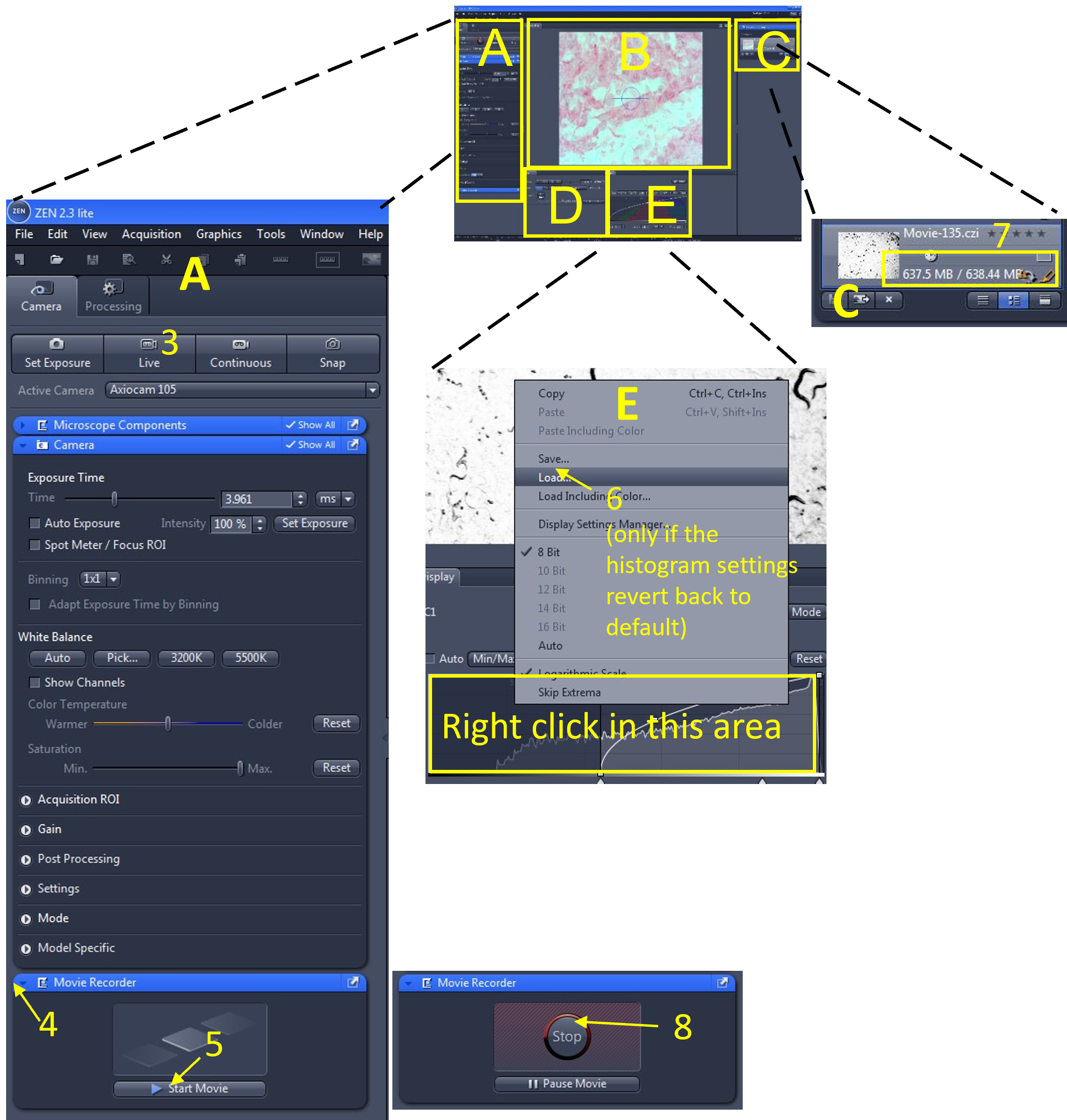
Zen Figure 11: Recording the video #1. - In the main tool area (A), turn off the Live view (3) by de-selecting the Live icon.
- Open the Movie Recorder menu (4) and click the Start Movie button (5) to begin recording the movie.
- Sometimes the histogram settings revert back to the default values when you start recording the video. You can quickly reload the histogram settings you previously saved by right clicking in the histogram display and loading the settings that you just saved (6).
- Look in the file and documents area (C) and monitor the size of the video file being recorded (7). Keep all video files <2.5 GB.
- When you are done recording (or the file size is approaching 2.5 GB), select stop (8) from the movie recorder menu.
ADDING A RELATIVE TIME GRAPHIC TO YOUR VIDEO AND CALCULATING FRAME RATE:
- Add a relative time graphic to your video to accurately determine the length of time between any two frames and calculate the frame rate (frames per second). This will allow you to export the video with the correct framerate.
- Select the video file you just recorded from the documents and files area (C).
- In the image/video editing area (D) select the dimensions menu (1), and make sure the slidebar is on the first frame of the video (2).
- Open the graphics menu (3) and select the relative time graphic (4). The relative time for each frame will appear on the top left of the video (5) that is currently displayed in the image display area (B). You can move the text box displaying the relative time graphic by clicking and holding to drag it around.
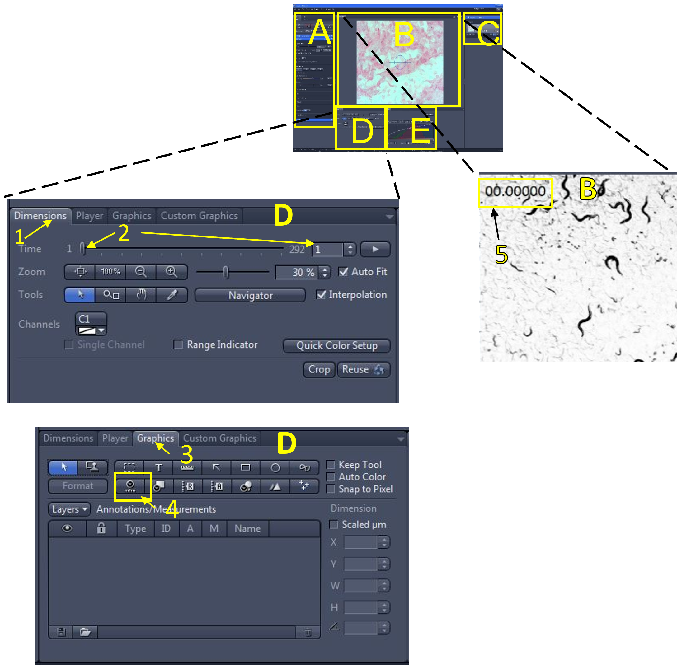
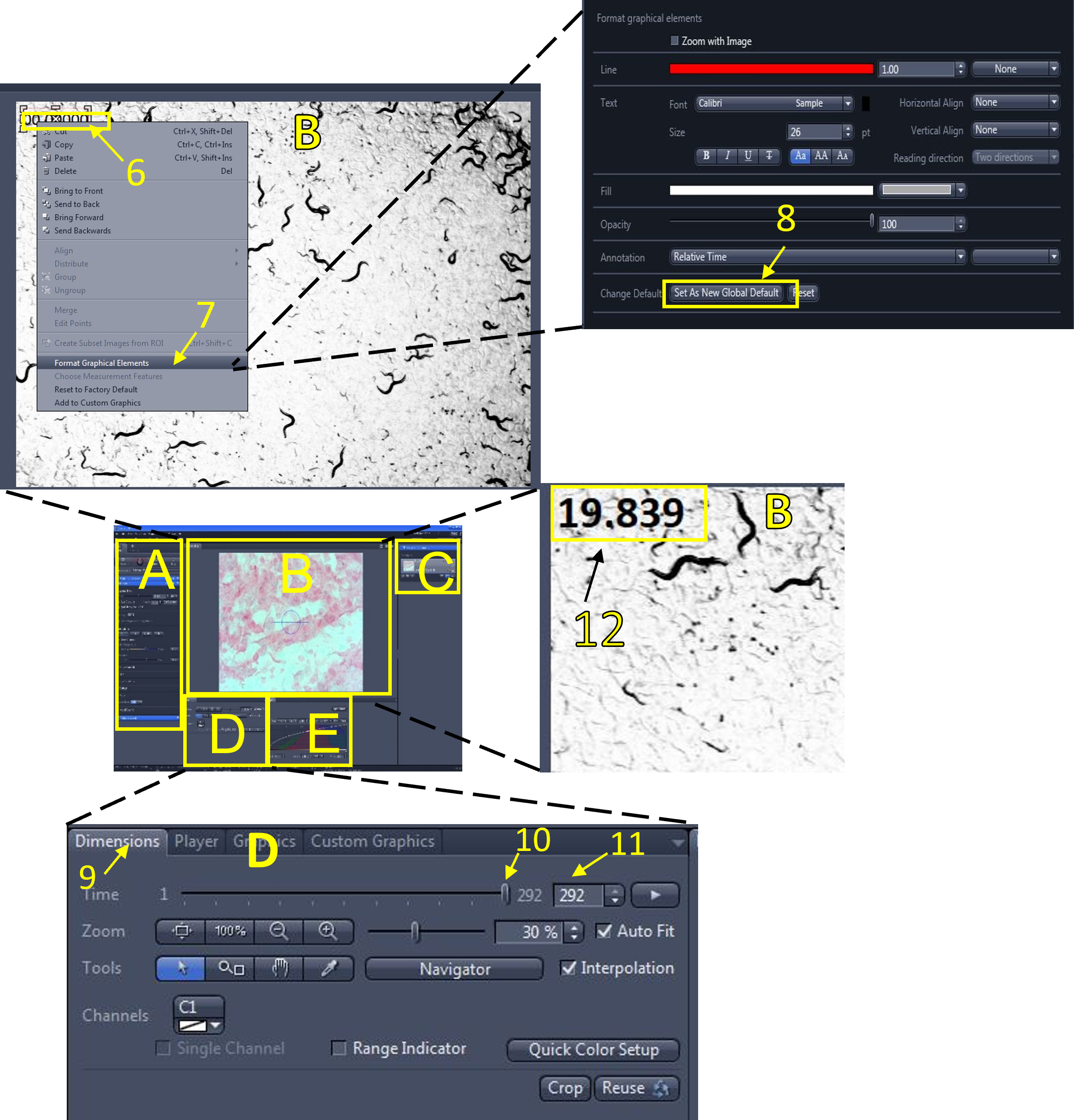
Zen Figure 13: Adding a relative time graphic. - To format the relative time graphic (if needed), right click the graphic currently displayed in the video (6), select format graphical elements (7), and change the formatting options (font size, colour etc.)You can save these options as the new default by selecting set as new default (8).
- In the video/image editing area (D), click the dimensions menu (9), and use the slide bar (10) or enter a frame # (11) to move between the frames of your video. The relative time of each frame will be displayed (frame 1 is time = 0 sec). Move the slide bar to the last frame (292nd frame in this example) and look at the relative time being displayed (12). It reads 19.839 seconds in this example. Calculate the frame rate in frames per second (FBS) by dividing the total # of frames (292) by the relative time displayed on the last frame (19.839 sec):
- (292/19.839 = 14.72 FPS)
SAVE AND EXPORT THE VIDEO
- Save each video immediately after you take it in case the software crashes.
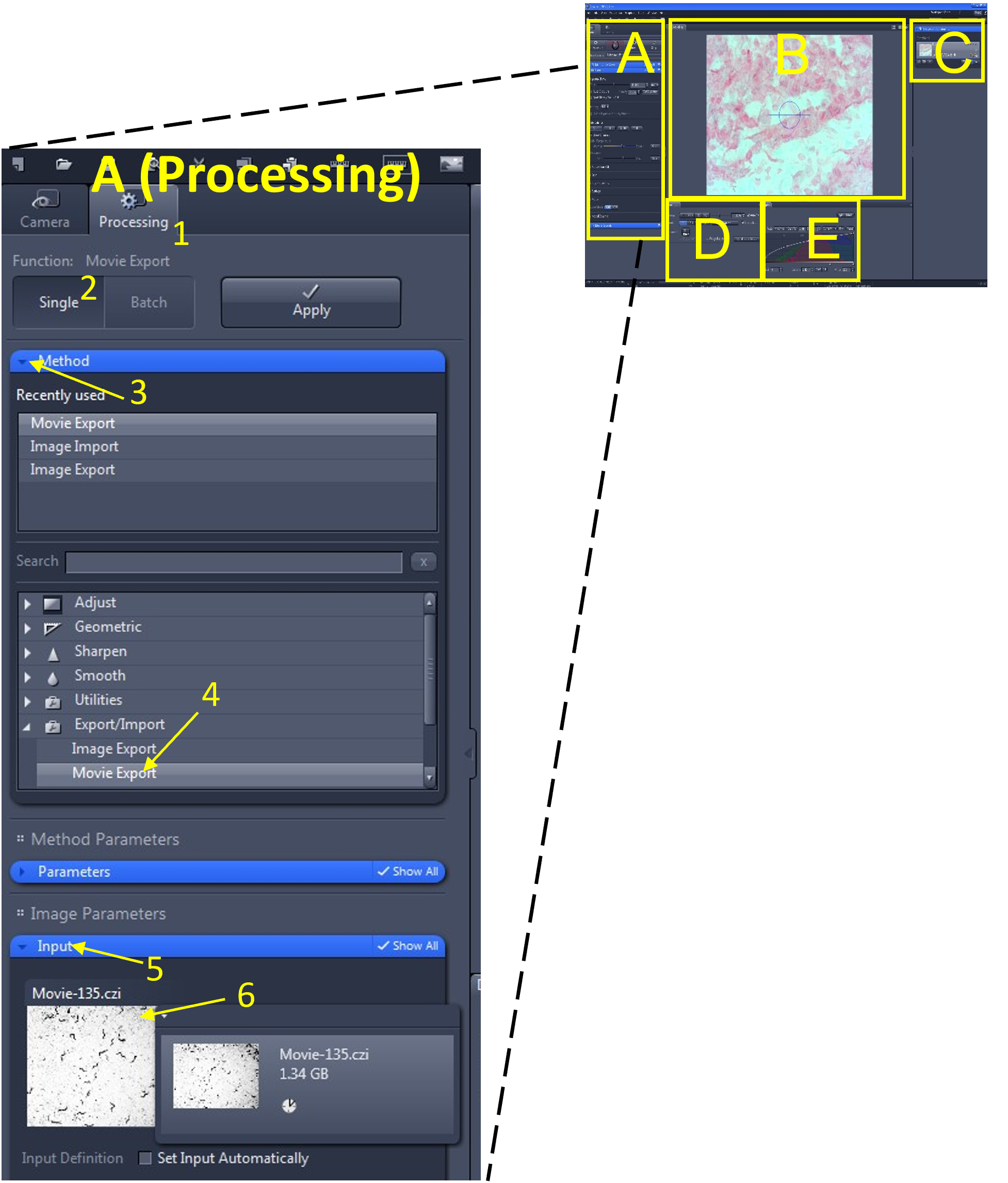
- In the main tool area (A), select the processing menu (1) and select single (2).
- In the method menu (3), find and select Movie Export (4) from the export/import submenu.
- Under the Input menu (5) select the video you wish to export (6). Alternatively, you may also click and drag the video from the Images and Documents area (C) into the input box.
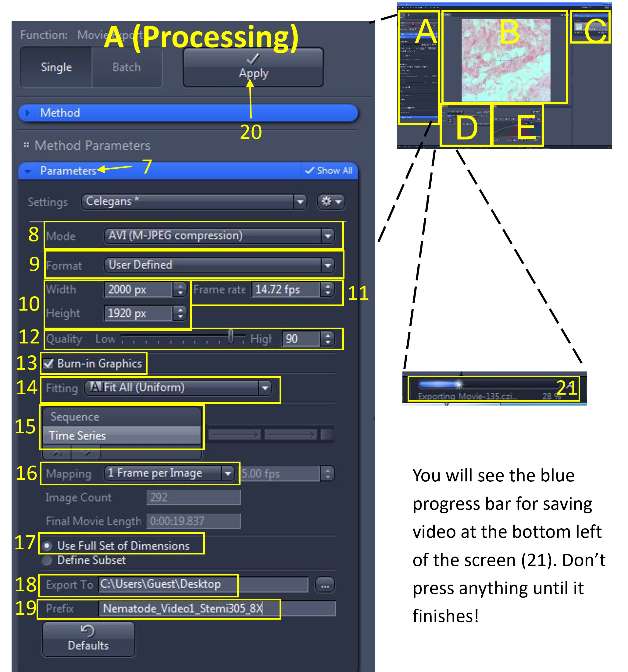
Zen Figure 15: Save and export the video #1. - Under the Parameters menu (7), use the following settings:
- Mode (8): AVI (M-JPEG compression)
- Format (9): User Defined
- Width and Height (10): Leave as they appear (the original size)
- Frame Rate (11): Enter the frame rate you calculated for the video
- Quality (12): 90 (default)
- Burn in Graphics (13): check box selected
- Fitting (14): Fit All (Uniform)
- Choose Time Series (15)
- Mapping (16): 1 frame per Image
- Choose Use full set of dimensions (17)
- Export to (18): select your group folder
- Prefix (19): Enter a name for the video (include tissue type, microscope used and total magnification e.g. Nematode_Video_Stemi305_8X_1)
- When you are ready to export, select the Apply button (20) at the top.
Part 6: Software and microscope shutdown
- Ensure all files are saved and uploaded to your Microsoft OneDrive folder as required. Do not save your files to a USB stick.
- Close the Zen application, allow for it to fully shut down, and log out of the computer.
- Remove and store the specimen, lower the microscope stand, and power off the microscope using the on/off switch.
- Return the workstation to the way you found it for the next lab group.
Note: It may take some time for the larger files to upload to the Drive, allocate time for video upload.
Appendix G: Virtual Microscope - Histological database exploration activity
During the first week of classes, we ask that you complete this virtual microscope activity using the 'OpenScience Laboratory - Histology & Histopathology' database. This module is optional, but will prepare you for working with microscopes in the lab space in the coming weeks, and will familiarize you with images of sectioned tissue, various structures and artifacts.
- Access the 'Histology & Histopathology: Virtual Microscope'
- This is an open-access interactive microscope tool made available by The Open University and The Wolfson Foundation. The accessible material is a collection of 320 annotated slides covering basic histology and histopathology, and is copyrighted. You will explore the virtual microscope and make observations about some slides during this activity.
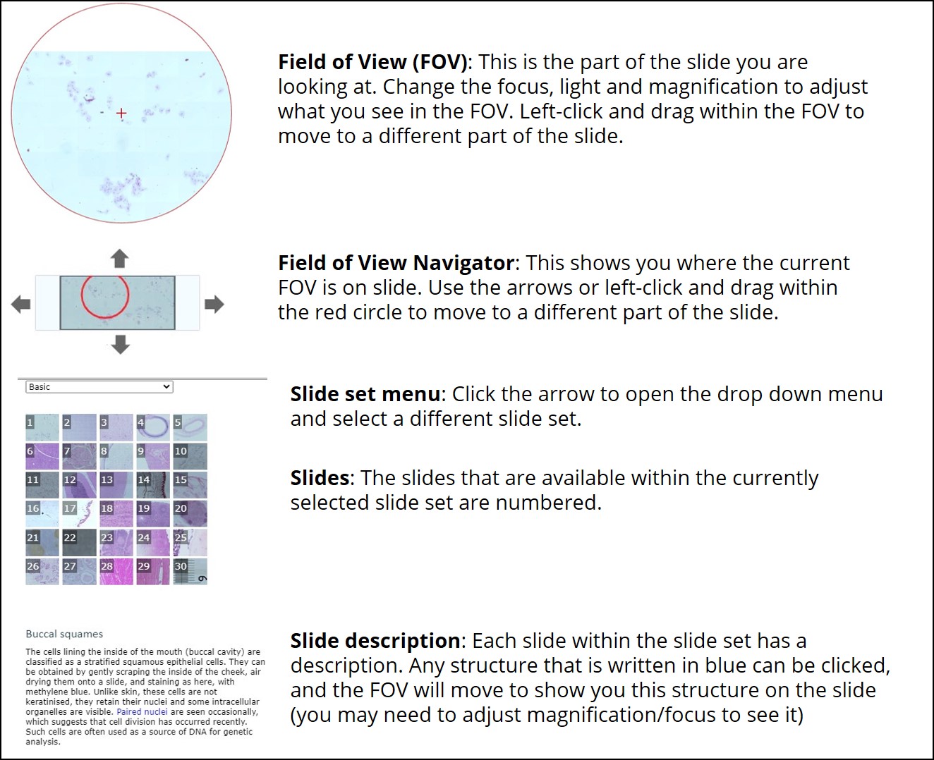
- The simulation opens up slide #1 (buccal squames) from the 'basic slide set'. At this point, it is an unfocused slide of “buccal squames,” which are cells that can be obtained by scraping the inside of your cheek. You may have tried an experiment like this in high school, where you collected tissue from the inside of your cheek in a biology class.
- You will see a number of settings on the left side of the simulation, described in figures 4 and 5. These are the same settings you will find on most microscopes in a research laboratory.
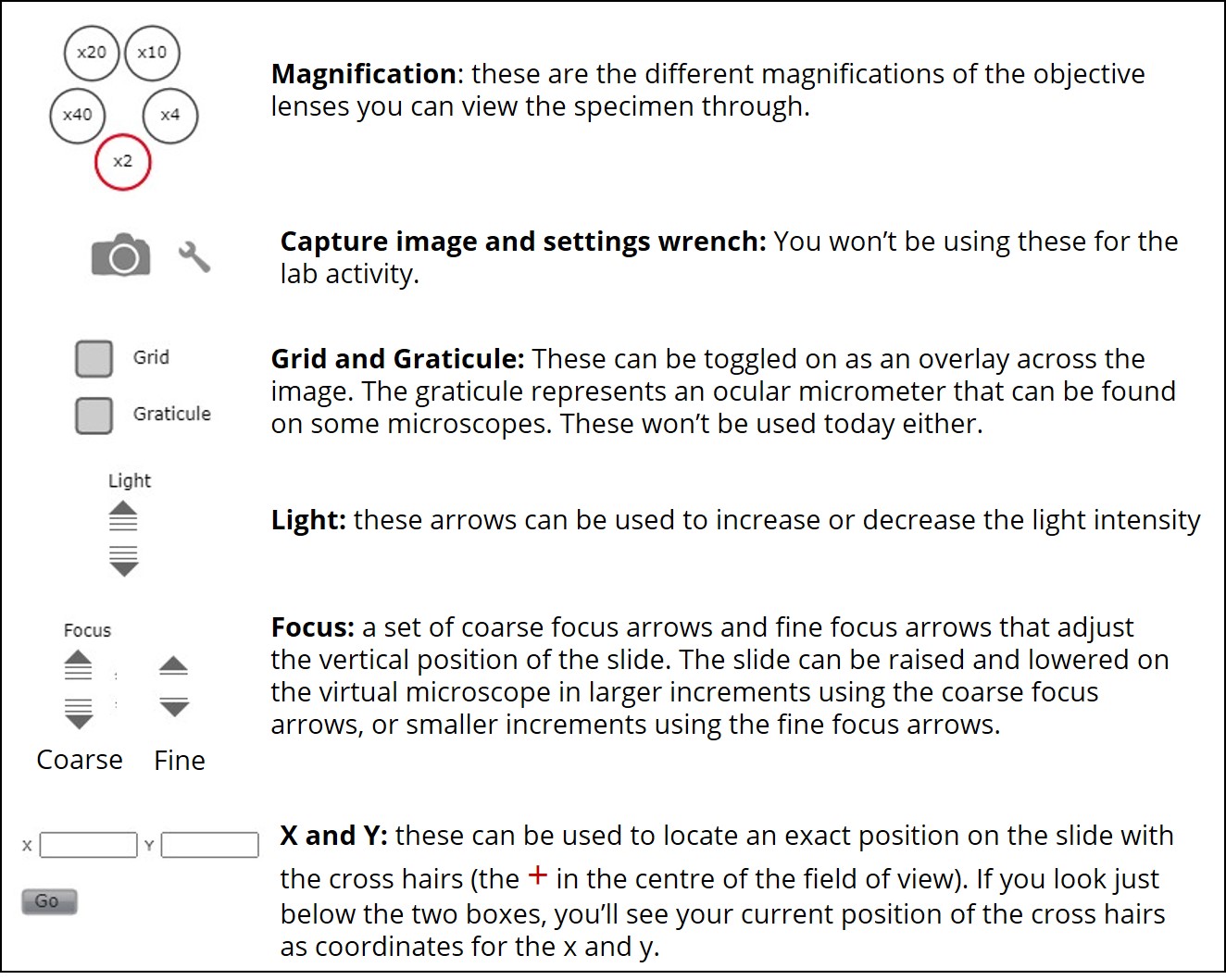
- Familiarize yourself with the settings buttons. First, use the coarse focus to bring the buccal cells into focus in the field of view.
- Next, find a nice clump of cells you would like to look at. Move your field of view by using the arrows around the slide at the bottom-centre of the simulation. Centre your crosshairs over the cells of interest.
- Increase your magnification to the next greatest lens (if you were at x2, increase to x4).
- Refocus your field of view using the fine focus arrows.
- Increase to the next magnification (x10).
- You may want to increase the light intensity as your magnification increases. This will help you see the cell membranes and fine features of the cellular structures.
- Make sure you have the 10X objective selected. Enter the following cross hair coordinates: X = 7213, Y = 3982. Click “Go.” How many cells are present in the clump your crosshairs are now centered on?
- In the top right corner of the simulation, there is a drop down menu to switch between different slide sets. Beneath this, there is a grid of the slides present in the current set. Select slide 17.
- You will note you have automatically been switched back to the lowest magnification. This is a best practice when working with a microscope. Always find your region of interest at lower magnification first, then focus and work your way up to higher magnifications incrementally.
- Focus the slide in the field of view. When focused, click the hyperlinked “epidermis” in the description of the slide at the right. This will align your crosshairs at the basal layer of the epidermis.
- Increase your magnification and adjust your focus incrementally until you are focused on this region of the slide at x20 magnification.
- What colour are the nuclei of the cells in the epidermis?
- Select slide 14.
- Adjust your focus and light intensity as required, and increase your magnification incrementally to x10.
- Familiarize yourself with the different layers of the skin by using the description of the slide at the right and the hyperlinked terms.
- Which cell layer is composed primarily of adipose tissue? Describe what this layer looks like on the slide.
- Use the dropdown menu at the top right to select the “skin” slide set. Select slide 3.
- This slide shows a sample of skin that was excised during wound healing. This sample does not match excision location of the previous slide, so we cannot directly compare the differences between the two, but there are some key differences that can be investigated by using the hyperlinks in the description.
- Move your field of view to the stratum corneum (recall, this is the layer of cell remnants outside of the epidermis, which provides the outermost layer of protection). Adjust your focus and light intensity as required, and incrementally increase the magnification to x10.
- Make a qualitative observation about the difference in the stratum corneum on this slide in comparison to the stratum corneum on the previous slide (slide #14 from the 'basic slide set').
- Use the dropdown menu at the top right to select the “stains and artefacts” slide set. Select slide 17.
- When a microtome is used to section tissue embedded in a paraffin block, the thin layers produced are in the range of 5-10 µm thick. This means the layers are very delicate, and artifacts can be produced quite easily when the layer of tissue is being mounted onto a slide and stained for imaging. This slide shows an example of an artifact called a fold.
- Using the light intensity arrows, the focus arrows, and the magnification lenses, find one part of the fold on this slide and focus on it at a magnification of x10. Observe the distortions caused by this fold, and how the cell structure is not preserved.
- Describe what could have caused this 'fold' artefact to occur.
- Feel free to explore the open-source database more. There are several slides that depict different cell types and many cases of pathological tissue samples that you may find interesting to look at.
