3.2 Logical and Lookup Functions
Learning Objectives
- Use and IF Function to make logical comparisons between a value and what you expect.
- Create a VLOOKUP calculation to look up information in a table.
- Understand error messages.
- Understand how to enter and format Date/Time Functions.
In addition to doing arithmetic, Excel can do other kinds of functions based on the data in your spreadsheet. In this section we will use an =IF function to determine whether a student is passing or failing the class. Then, we will use a =VLOOKUP function to determine what grade each student has earned.
IF Function
The IF function is one of the most popular functions in Excel. It allows you to make logical comparisons between a value and what you expect. In its simplest form, the IF function says something like:
If the value in a cell is what you expect (true) – do this. If not – do that.
The IF function has three arguments:
- Logical test – Here, we can test to see if the value in a selected cell is what we expect. You could use something like “B7=14” or “B7>12” or “B7<6”
- Value_if_true – If the requirements in the logical test are met – if B7 is equal to 14 – then it is said to be true. For this argument you can type text – “True”, or “On budget!” Or you could insert a calculation, like B7*2 (If B7 does equal 14, multiply it by 2). Or, if you want Excel to put nothing at all in the cell, type “” (two quotes).
- Value_if_false – If the requirements in the logical test are not met – if B7 does not equal 14 – then it is said to be false. You can enter the same instructions here as you did above. Let’s say that you type the double quotes here. Then, if B7 does not equal 14, nothing will be displayed in this cell.
In column Q we would like Excel to tell us whether a student is passing – or failing the class. If the student scores 70% or better, he/she will pass the class. But, if he/she scores less than 70%, he/she is failing.
- Make sure that Q5 is your active cell.
- On the Formulas tab, in the Function Library, find the IF function on the Logical pulldown menu (see Figure 3.9).
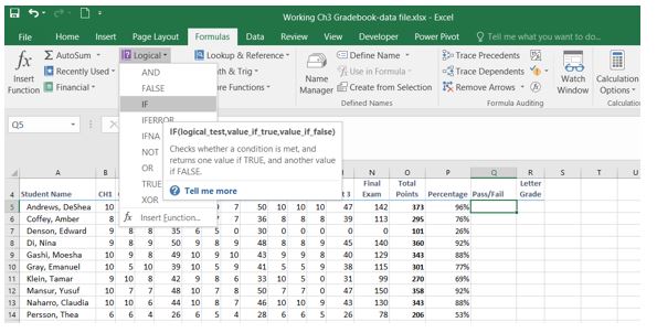
Figure 3.9 IF Function

Now you will see the IF Function dialog box, with a place to enter each of the three arguments.
- Click in the box for Logical Test. We need to test whether a student’s score is less than .7. So, in this box, type P5<.7
- Click in the box for Value_if_true. If the student’s score is less than .7, then they are failing the class. In this box, type Fail.
- Click in the box for Value_if_false. If the student’s score is NOT less than .7, then they are passing the class. In this box, type Pass.
- Make sure that your dialog box matches Figure 3.10.
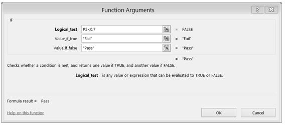
Figure 3.10 IF Function Dialog Box While we are here, let’s take a look at the dialog box. Notice that as you click in each box, Excel gives you a brief explanation of the contents (in the middle below the boxes.) In the lower left hand corner, you can see the results of the calculation. In this case DeShae is passing the class. Below that is a link to Help on this function. Selecting this link will take you to the Excel help for this function – with detailed information on how it works.
- Once you have typed in the required arguments and reviewed to make sure they are correct, press OK. (The text Pass should be displayed in Q5 because DeShae is passing the class.)
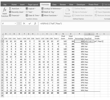
- Use the Fill handle to copy the IF function down through row 24.
- Click on Q5. When you look in the formula bar, you will see the IF calculation: =IF(P5<0.7,”Fail”,”Pass”) (see Figure 3.11).

VLOOKUP Function
You need to use a VLOOKUP function to look up information in a table. Sometimes that table is on a different sheet in your workbook. Sometimes it is in another file entirely. In this case, we need to know what grade each student is getting based on their percentage score. You will find the table that defines the scores and the grades in A28:B32.
There are four pieces of information that you will need in order to build the VLOOKUP syntax. These are the four arguments of a VLOOKUP function:
- The value you want to look up, also called the Lookup_value. In our example, the lookup value will be the student’s percentage score in column P.
- The Table_array is the range (table) where the lookup values and the values you want returned by the function are located. In our example, this is the table of percentages and corresponding letter grades in the range A28:B32. The lookup value should always be in the first column in the table array for VLOOKUP to work correctly. For example, in our table_array the lookup value is in cell A28, so the range should start with A.
- The Col_index_num is the column number in the range that contains the value to return. In our example, when you specify A28:B32 as the Table_array range, you should count A as the first column (1), B as the second column (2), and so on. You will enter the appropriate column number in this box as 1, 2, or 3 and so on.
- In the Range_lookup, you can optionally specify TRUE if you want an approximate match or FALSE if you want an exact match of the return value. If you leave this blank, the default value will always be TRUE, or approximate match.
Let’s create the VLOOKUP to display the correct Letter Grade in column R.
- Make sure that R5 is your active cell.
- On the Formulas tab, in the Function Library, find the VLOOKUP function on the Lookup & Reference pull-down menu (see Figure 3.12).
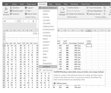
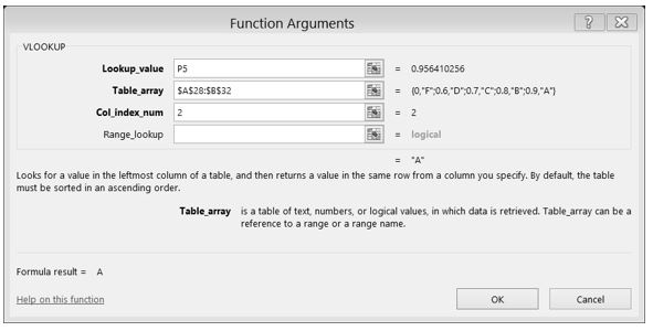
Figure 3.12 VLOOKUP Function - Fill in the dialog box so that it looks like the image in Figure 3.13.
- Lookup_value – In this case, we will use the Percentage score. So, P5 for the first look up value.
- Table_array – This is the range that contains the value you want returned by the function. In this case, that range is A28:B32. Note that this range does NOT include the label in row 27; just the actual data. The cell references for the Table_array need to be absolute – $A$28:$B$32. When we copy this function to the other cells, we do not want these cell references to change. It should always be $A$28:$B$32.
- Col_index_number – This is the column in the table array range that includes the information that we are looking up. In our case, the actual grades are in the 2nd column of the range. So, the column index will be 2.
- Range_lookup – In some cases, you will need something in the Range_lookup box. Since we are looking for an approximate match for the percentages, we want the default value of TRUE, so we do not need to enter anything for this argument.
- While you are in the dialog box, be sure to look at all the helpful definitions that Excel offers.
- When you have filled in the dialog box, press OK.
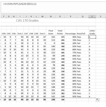
- The calculation you will see in the formula bar is: =VLOOKUP(P5,$A$28:$B$32,2)
- Use the fill handle to copy the function down through row 24. The results displayed should match Figure 3.14.

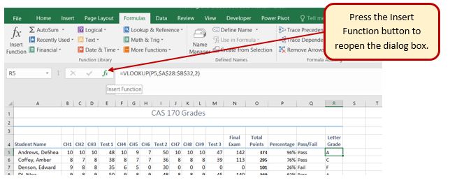
Note: What if it didn’t work? What if you get a result different from the one predicted? In this case, either you have made a previous error, resulting in different % scores than this exercise anticipated, or you made a mistake entering your VLOOKUP function.
To make repairs in the function, make sure that R5 is your active cell. On the Formula bar, press the Insert Function button (see Figure 3.15). That will reopen the dialog box so you can make your repairs. Did you forget to make the cell references for the Table_array absolute? Did you use the wrong cell for the Lookup_value? Press OK when you are done and recopy the corrected function.
Error Messages
Sometimes Excel notices that you have made errors in your calculations before you do. In those cases Excel alerts you with some slightly mysterious error messages. A list of common error messages can be found in Table 3.1 below.
Table 3.1 – Common Error Messages
| Message | What Went Wrong |
| #DIV/0! | You tried to divide a number by a zero (0) or an empty cell. |
| #NAME | You used a cell range name in the formula, but the name isn’t defined. Sometimes this error occurs because you type the name incorrectly. |
| #N/A | The formula refers to an empty cell, so no data is available for computing the formula. Sometimes people enter N/A in a cell as a placeholder to signal the fact that data isn’t entered yet. Revise the formula or enter a number or formula in the empty cells. |
| #NULL | The formula refers to a cell range that Excel can’t understand. Make sure that the range is entered correctly. |
| #NUM | An argument you use in your formula is invalid. |
| #REF | The cell or range of cells that the formula refers to aren’t there. |
| #VALUE | The formula includes a function that was used incorrectly, takes an invalid argument, or is misspelled. Make sure that the function uses the right argument and is spelled correctly. |
This table was copied from the internet. Look here for additional information.
http://www.dummies.com/software/microsoft-office/excel/how-to-detect-and-correct-formula-errors-in-excel-2016/
Date Functions
Very often dates and times are an important part of Excel data. Numbers that are correct today may not be accurate tomorrow. So, it is frequently useful to include dates and times on your spreadsheets.
These dates and times fall into two categories – ones that:
- Remain the same. For instance, if a spreadsheet includes data for May 15th, you don’t want the date to change each time you re-open the spreadsheet.
- Change to reflect the current date/time. When it is important to have the current date or time on a spreadsheet, you want Excel to update the information regularly.
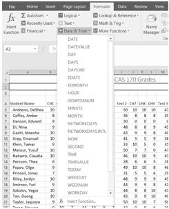
Take a look at the list of Date and Time functions offered in the Function Library on the Formulas tab (see Figure 3.16).
For our gradebook, we want the date and time to be displayed in A2, and it needs to update whenever the workbook file is opened.
- Make A2 your active cell. Notice that A2 extends all the way from column A to Column R. Previously, someone has used the Merge & Center tool on this cell to make it match the title above.
- On the Formulas tab, in the Function Library, select NOW from the Date & Time drop-down list and then click OK.
- The result you will see in the formula bar is: =NOW(). The result you will see in A2 depends on the current date and time.The NOW function is a very handy function. It takes no arguments and is Volatile! That is not as alarming as it may seem. This just means that you don’t need to give it any more information to do its job and that your results will change frequently.You can update the date and time whenever you want – you don’t have to wait until you open the workbook again.
- Make sure that A1 is your active cell and press the F9 function key (along the top of your keyboard.) The time will update.
Excel will update this field independently whenever you save and re-open the file, or print it. It may happen more frequently than that – depending on how you have set this up in your installation of Excel.
Another variation of the current date is the TODAY function. Let’s try that one next.
- Make sure A2 is your active cell. Press Delete to remove the NOW function.
- From the Date & Time drop-down list in the Function Library on the Formulas tab (see Figure 3.16), select TODAY and then click OK.
- The result you will see in the formula bar is: =TODAY(). The result you will see in A2 depends on the current date.Since we haven’t asked for the time, the time you are seeing is likely 12:00. That is not very helpful so we need to change the format of the date.
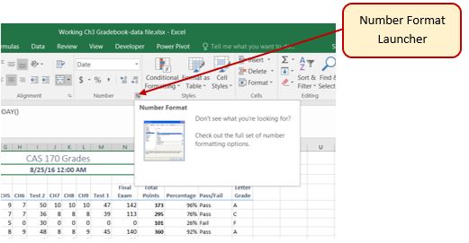
- On the Home tab, in the Number group, press the Number Format Launch button (see Figure 3.17).
- In the Format Cells dialog box, click the Number tab. Choose the Date category and select Wednesday, March 14, 2012 (this format is called Long Date).
- The current day and date will display in A2.
Keyboard Shortcuts
Sometimes you want the date or the time to show up in your spreadsheet, but you don’t want it to change. You can simply type in the date or time. Or, you can use shortcut keys.
- CTRL; (semi colon) will bring you the current date
- CTRL: (colon or CTRL SHIFT ; ) will bring you the current time.
Key Takeaways
- Functions don’t always have to be about arithmetic. Excel provides functions that will help you perform logical evaluations, look things up, and work with dates and times.
- Excel displays error messages when your formulas and functions are not constructed properly.
Attribution
3.2 Logical and Lookup Functions by Noreen Brown and Mary Schatz, Portland Community College, is licensed under CC BY 4.0
