Maheshwar Panday
Wisconsin Breast Cancer Data: Analyzing High Dimensional Data
You are a pathologist and have taken the measurements of 569 nuclei of cells from needle aspirates of breast tissue masses. Samples come from either benign (B) or malignant (M) masses. You would like to perform an analysis of the cell shapes and sizes between the malignant and benign cells to better understand the differences between them. You would also like to explore using machine learning to see how well simple clustering algorithms can identify benign cells from malignant ones based SOLELY on their size and shape features. Using the Wisconsin Breast Cancer Dataset
———– Text from Kaggle ——————– The breast cancer data includes 569 examples of cancer biopsies, each with 32 features. One feature is an identification number, another is the cancer diagnosis and 30 are numeric-valued laboratory measurements. The diagnosis is coded as “M” to indicate malignant or “B” to indicate benign.
The other 30 numeric measurements comprise the mean, standard error and worst (i.e. largest) value for 10 different characteristics of the digitized cell nuclei, which are as follows:-
Radius Texture Perimeter Area Smoothness Compactness Concavity Concave Points Symmetry Fractal dimension ——————– Dataset Link Below ————— Breast Cancer Dataset available from : https://archive.ics.uci.edu/dataset/17/breast+cancer+wisconsin+diagnostic
for further reading on the Wisconsin Breast Cancer Dataset,specifically how each of the features in this dataset were calculated, please consult:
Street, W.N., Wolberg, W.H., & Mangasarian, O.L. (1993). Nuclear feature extraction for breast tumor diagnosis. Electronic imaging.
(1) Loading packages for statistics, clustering, dimensionality reduction and data visualisation
Install and load the following packages into R
library(dabestr) # estimation statistics
library(ggplot2) # plotting and data visualisation
library(pheatmap) # generating a heatmap
library(tidyverse) # data handling
library(dplyr) # data handling
library(stats) # basic statistics
library(RColorBrewer) # colour palettes and plot aesthetic controls
library(Rtsne) # for performing T-distributed stochastic neighbour embedding (tsne)
Download the dataset from the UCI Machine Learning Repository. Load the csv file of measurements into RStudio
BreastCancer.Data <- read.csv("WisconsinBreastCancerData.csv")
BreastCancer.Data$X <- NULL
print (head(BreastCancer.Data))
(3) Prepare the dataframes for tsne and subsequent clustering
The entire BreastCancer.Data dataframe is structured such that each row is a cell and each column is a parameter. However, there are certain columns that are not features (quantitative descriptions of the cells). When a column is not a feature, it’s a label. Labels are ways to identify or tag specific cells once we understand how they are characterised by their features.
Before we can explore the dataset, we need to separate the labels from the features.There are two columns in the dataframe that label the cells – id -> the unique identification number assigned to a cell – diagnosis -> whether the cell is from a benign (B) or malignant (M) Sample)
The remaining columns are features that serve as quantitative descriptions of the cell sizes and shapes
- Your first task with these data is to subset the entire Breast Cancer Dataframe into two dataframes
- Diagnostic.Labels – which will contain the labels
- Diagnostic.Features – which will contain the features
- Because the magnitudes of the measures range over difference scales, you need to bring your data into a common space to allow for variations and differences to become apparent across features for the entire dataset. Z-score your dataset using the scale() operation in R on your Diagnostic.Features
## ---------------------------------------- ##
##### Setting features apart from labels #####
## ---------------------------------------- ##

# labels dataframe - contains the unique identifier and the diagnosis)
Diagnostic.Labels <- select(BreastCancer.Data, id, diagnosis)

# features dataframe - all the columns that are not identifiers are the measured features that characterise the tissue mass - specifically the characterizing the nuclei present.
feature.columns <- setdiff (colnames(BreastCancer.Data), colnames(Diagnostic.Labels))
Diagnostic.Features <- BreastCancer.Data[, feature.columns]

# create a z-scored version of the features
Diagnostic.Features.Scored <- scale(Diagnostic.Features)

# print (head(Diagnostic.Features.Scored))

view(Diagnostic.Features.Scored)
print (colnames(Diagnostic.Features.Scored)
(4) Explore the dataset using tsne
Tsne or T-distributed Stochastic Neighbour Embedding is a technique used to visualise high-dimensional data in 2 dimensions. Termed a dimensionality-reduction method, it allows us to explore the data one feature at a time. In this breast cancer dataset, there are 32 measures that describe the size, shape, and texture of masses in breast tissue that then go on to be either benign (B) or malignant (M).
For further reading on T-sne, please consult : Van der Maaten, L., Hinton, G. Visualizing Data using T-sne. Journal of Machine Learning Research 9 (2008) 2579-2605
Let’s use tsne to visualise how these features are distributed across the dataset.
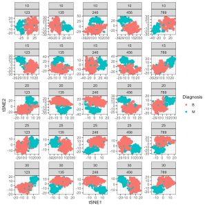
N.B. I ran this for loop of seed by perplexity combinations because it is important to test these parameters when wrorking with T-sne. The perplexity controls how much of the local vs. global data structure elements contribute to the final visualisation as the data pass through dimensionality reduction. Variations in perplexity for the same random seed can have very dramatic effects on the final visualisation despite the data not changing.
# Define your perplexities and seeds
perplexities <- c(10, 15, 20, 25, 30)
seeds <- c(123, 456, 789, 246, 135  )

# Create an empty dataframe to store the t-SNE components
tsne_data <- data.frame()

# Iterate over each combination of perplexity and seed
for (i in 1:length(perplexities)) {
  for (j in 1:length(seeds)) {
    # Perform t-SNE with the current perplexity and seed
    tsne_model <- Rtsne(Diagnostic.Features.Scored, perplexity = perplexities[i], seed = seeds[j])

    # Create a dataframe for the t-SNE components
    tsne_temp <- data.frame(
      tSNE1 = tsne_model$Y[, 1],
      tSNE2 = tsne_model$Y[, 2],
      Perplexity = perplexities[i],
      Seed = seeds[j],
      Diagnosis = Diagnostic.Labels$diagnosis
    )

    # Append the data to the main dataframe
    tsne_data <- rbind(tsne_data, tsne_temp)
  }
}


# Create the plot
tsne.stampcollection <- ggplot(tsne_data, aes(x = tSNE1, y = tSNE2, colour = Diagnosis)) +
  geom_point() +
  facet_wrap(Perplexity ~ Seed, scales = "free") +
  theme_bw()
(4) Student exercise – tsne to explore benign vs malignant cells using dimensionality reduction
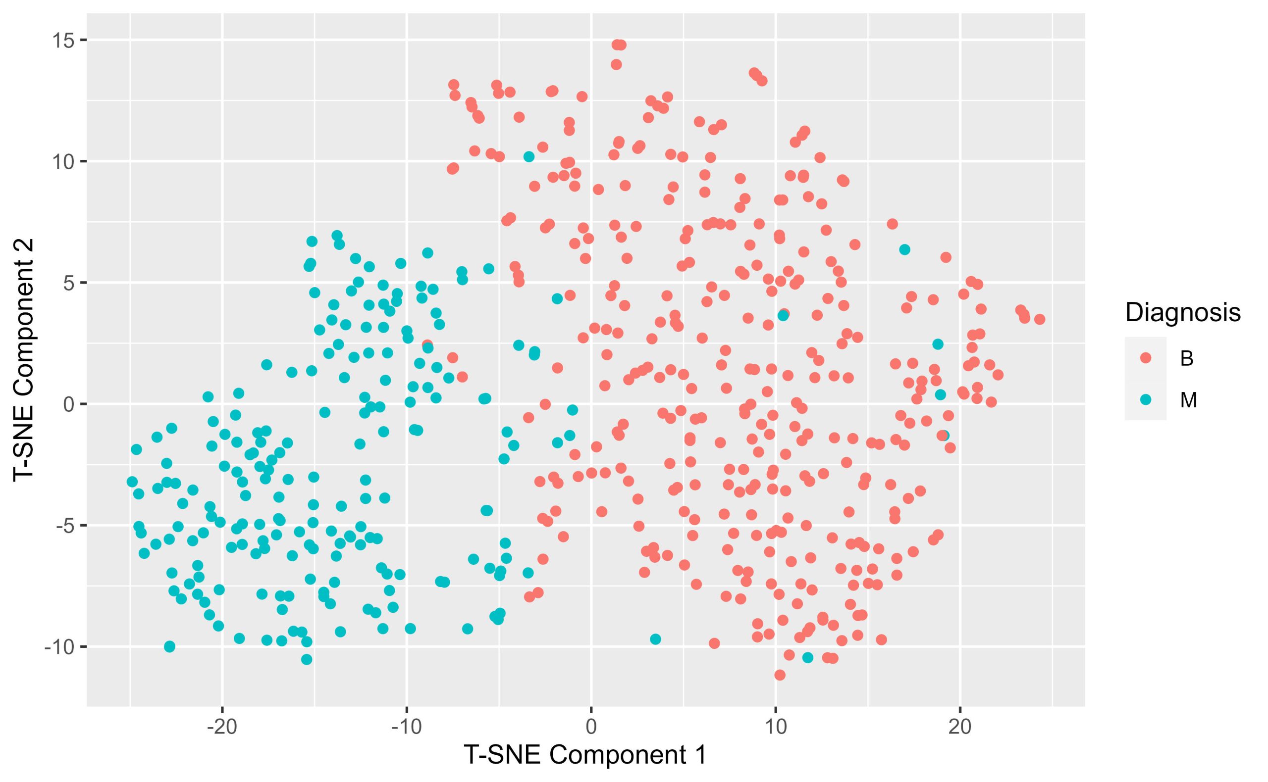
Use the following parameters in your initial tsne: – seed <- 789 – perplexity <- 30
Construct a T-sne map of the Diagnostic.Features dataframe. Plot the resulting T-sne map using ggplot making sure to colour the points by their diagnosis label. What do you notice about the T-sne map when it’s annotated by diagnosis?
As an exercise – vary the perplexity for the seed of 789, try ranging from 10 to 50 by skips of 10. What do you notice about the T-sne map as you vary the perplexity? What do you think the perplexity parameter controls in the T-sne algorithm?
# Set your perplexity and seed
set.seed (789)
perplexity <- 30
seed <- 789

# Perform t-SNE with the specified perplexity and seed
tsne_model <- Rtsne(Diagnostic.Features.Scored, perplexity = perplexity, seed = seed)

# Create a dataframe for the t-SNE components
tsne_data <- data.frame(
  tSNE1 = tsne_model$Y[, 1],
  tSNE2 = tsne_model$Y[, 2],
  Diagnosis = Diagnostic.Labels$diagnosis  # Add the diagnosis column
)

# Load ggplot2
library(ggplot2)

# Create the plot
tsne.by.diagnosis <- ggplot(tsne_data, aes(x = tSNE1, y = tSNE2, colour = Diagnosis)) +
  geom_point() +
  labs( x = "T-SNE Component 1", y= "T-SNE Component 2")
  theme_bw()

# Print the plot
print(tsne.by.diagnosis)
(5) Hierarchical clustering of malignant samples
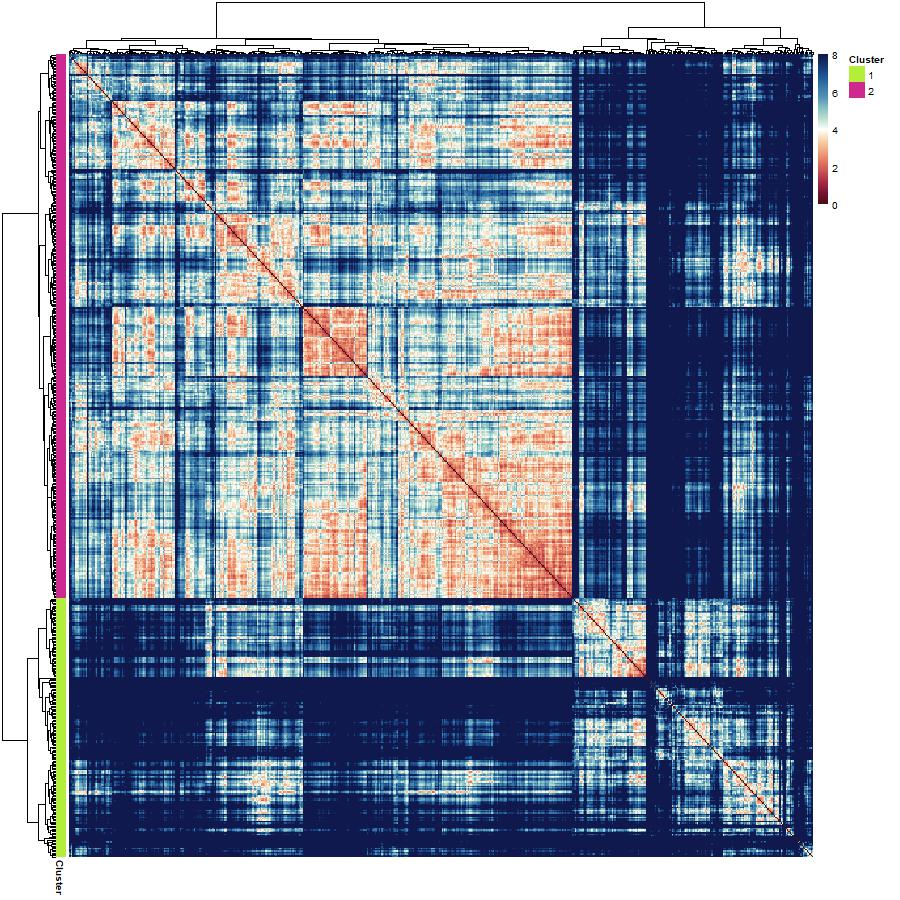
What if there were a way to readily identify cells as being benign or malignant depending on their size and shape parameters? Clustering algorithms are an example of a data-driven approach to grouping your data together based on the patterns present in the features. Of course, the data contain labels, but what if you clustered on the feature values, the measurements, without providing any information about the cell diagnosis? Select 2 clusters – we want to see whether hierarchical clustering separates benign vs malignant cells based on their shapes and size information only.
The steps to performing hierarchical clustering are as follows : 1.construct a dissimilarity matrix of the z-scored features. Use Euclidean Distances 2.call the hclust function on the dissimilarity matrix and specify the method is ward.D2 3.annotate the dendrogram to show where the data are partitioned into clusters 4. visualise the results of your clustering by constructing a heatmap of the dissimilarity matrix organised with an annotated surrounded dendrogram.
## ----------------------------------------------------- ##
#### dissimilarity matrix and hierarchical clustering #####
## ----------------------------------------------------- ##
# set the number of clusters
num.clusters <- 2


# construct a pairwise dissimilarity matrix using euclidean distances
dissimilarity.matrix <- dist(Diagnostic.Features.Scored, method = "euclidean")
# hierarchical clustering with Wthe ward.D2 algorithm
h.clusters <- hclust(dissimilarity.matrix, method = "ward.D2")
# cut the dendrogram into k clusters
clusters <- cutree(h.clusters, k = num.clusters)

## --------------------------------------------------- ##
##### Preparing Dataframe for Downstream Statistics #####
## --------------------------------------------------- ##

# create a dataframe of identifiers and z-scored features
All.Samples.zscored <- cbind(Diagnostic.Labels,
                                   Diagnostic.Features.Scored)
# append the clusters to the dataframe
All.Samples.zscored$hclust_clusters <- clusters
# view(Malignant.Samples.zscored) # inspection step


##--------------------------------------- ##
##### Annotating the HClust Dendrogram #####
##--------------------------------------- ##
# create an annotation dataframe
annotation.df <- data.frame(Cluster = as.factor(clusters))
rownames(annotation.df) <- rownames(Diagnostic.Features)
# apply a colour palette to the annotations on the dendrogram
# colour palette for the k clusters
k.cluster.colourpalette <- c("olivedrab2", "maroon3")
# colour mapping
colourmapping <- setNames(k.cluster.colourpalette, levels (annotation.df$Cluster))
# make a list of annotation colours
annotation.colours = list(Cluster = k.cluster.colourpalette)
# match the names of the annotation colours to the cluster levels ( 1-8)
names(annotation.colours$Cluster) <- levels(annotation.df$Cluster)


## ----------------------------------------- ##
##### visualising clustering in a heatmap #####
## ----------------------------------------- ##
# set a colour palette
# diverging - spectral
div.spectral.red.blue <- c("#4a100e", "#731331", "#a52747", "#c65154",  "#e47961", "#f0a882", "#fad4ac", "#ffffff",
                           "#bce2cf", "#89c0c4", "#5793b9", "#397aa8",  "#1c5796", "#163771", "#10194d" )
div.spectral.blue.red <- rev(div.spectral.red.blue)
# interpolate the colours for continuous scales
continuous.spectral.redblue <- colorRampPalette(div.spectral.red.blue) (256)
continuous.spectral.bluered <- colorRampPalette(div.spectral.blue.red)(256)


# set the breaks in the colour scale
palette.breaks <- seq(from= 0, to = 8, length.out = length (continuous.spectral.redblue) + 1)


# generate the heatmap
hclust.dissimilarity.heatmap <- pheatmap(dissimilarity.matrix,
                                               cluster_rows = h.clusters,
                                               cluster_cols = h.clusters,
                                               annotation_row = annotation.df,
                                               # annotation_col = annotation.df,
                                               annotation_colors = annotation.colours,
                                               color = continuous.spectral.redblue,
                                               breaks = palette.breaks)
(6) Inspecting the results of your hierarchical clustering :
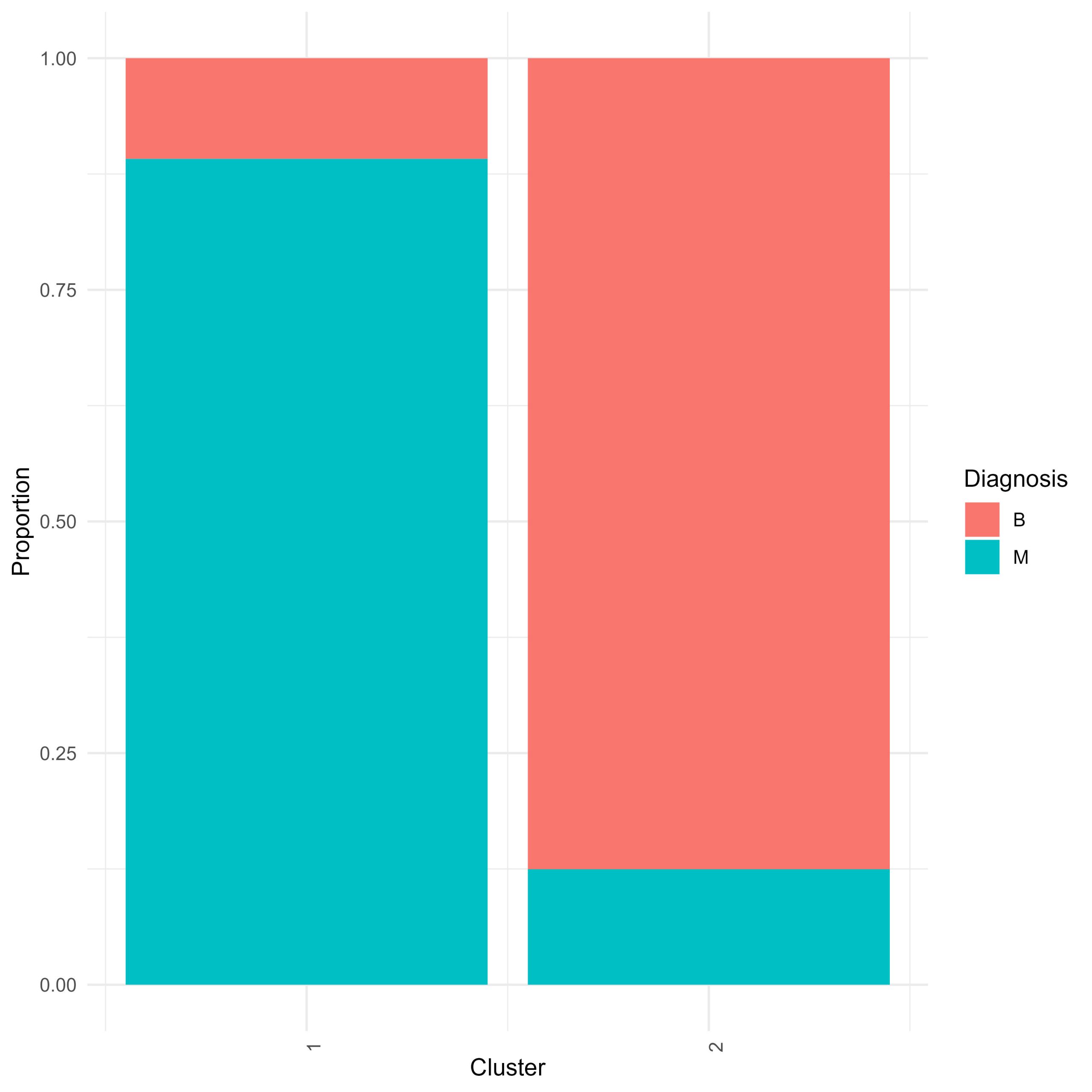
You have just produced a hierarchical clustering result. You can visualise the clustering with a heatmap with an annotated surrounding dendrogram, but that doesn’t tell you about which cells were relegated into which cluster. You can also produce a stacked proportion barplot that shows you the proportion of benign and malignant cells in a cluster.
- prepare a dataframe of proportions – group the data by cluster and diagnosis and calculate percentages.
- prepare a stacked proportion barplot using ggplot and geom_bar element. Based on the results of the clustering how well did hierarchical clustering do in clustering benign and malignant cells apart from each other?
library(dplyr)

# Calculate proportions of benign and malignant cells by cluster
# you can use the pipe operator to nest a series of operations to be performed to the dataframe of origin
All.Samples.zscored.grouped <- All.Samples.zscored %>%
  group_by(hclust_clusters, diagnosis) %>%
  summarise(n = n()) %>%
  mutate(freq = n / sum(n))
view (All.Samples.zscored.grouped)

# Prepare a stacked proportion barplot


Hclust.barplot <- ggplot(All.Samples.zscored.grouped, aes(fill=diagnosis, y=freq, x=hclust_clusters)) +
  geom_bar(position="fill", stat="identity") +
  theme_minimal() +
  labs(x="Cluster", y="Proportion", fill="Diagnosis") +
  scale_x_continuous(breaks = c(1,2))+
  theme(axis.text.x = element_text(angle = 90, hjust = 1))
– Student Question – Across the features in your dataframe there are patterns in those data that can distinguish benign from malignant cells. You want to assess how different the benign and malignant cells are.
(7) Performing Estimation Statistics by Diagnostic Label
Estimation statistics are an alternative framework for statistical analysis that do not depend on p-values or significance testing. Instead they show the data, the distributions and their unpaired median differences along with bootstrapped 95% confidence intervals. This framework allows you to see your data and make assessments of difference/no difference without significance testing. It is a powerful framework that makes statistical inference visually accessible and frankly, beautiful!
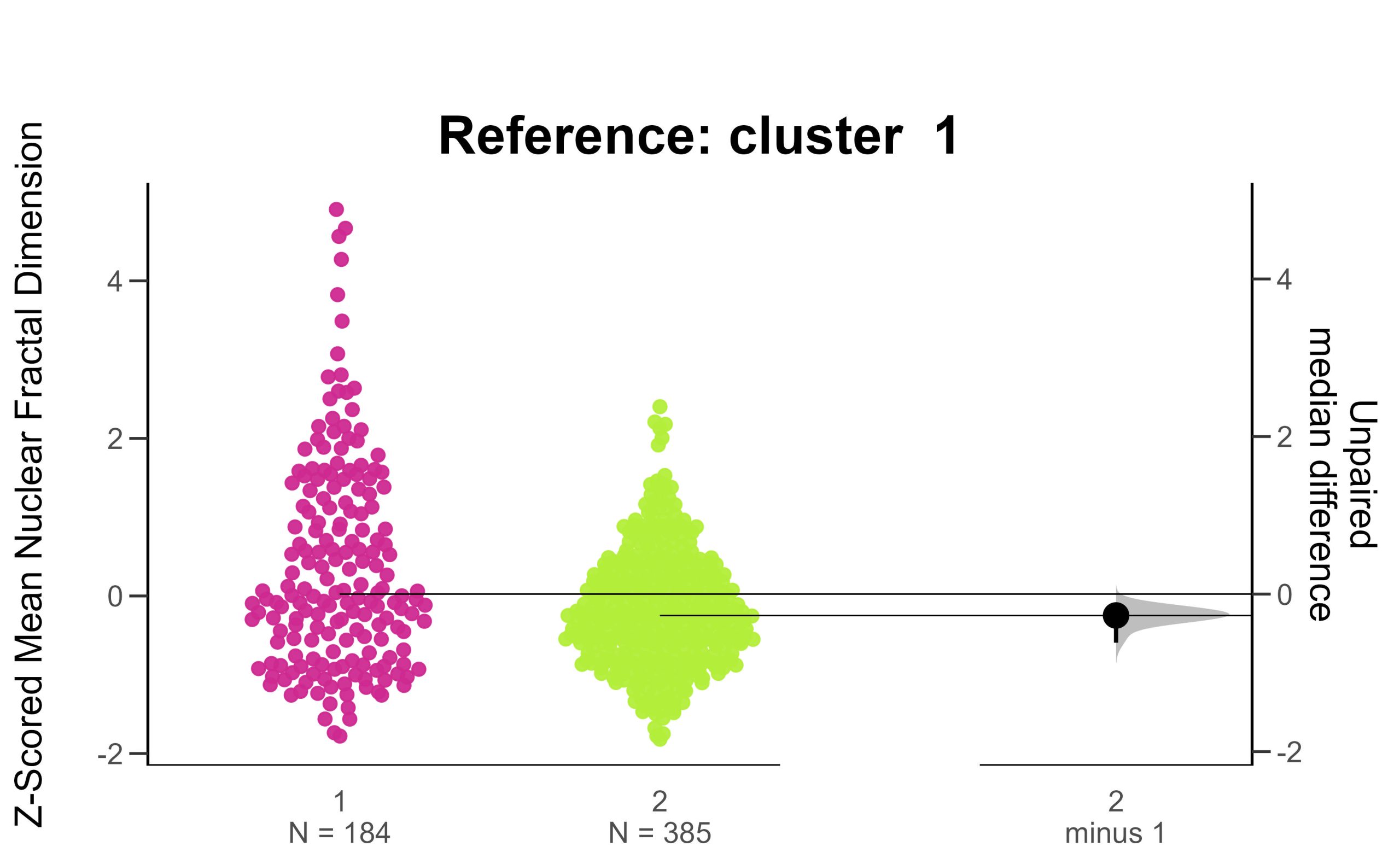
(8) Performing Estimation Statistics by Hierarchical Cluster
The previous estimation statistics were applied to the cells categorised by diagnostic label – to assess for differences in features between benign and malignant cells. This time, repeat the same estimation statistics framework and look at the same features, but apply estimation statistics to the clusters instead. How do the estimation plots by cluster compare to the estimation plots by diagnostic label?
For further reading on estimation statistics please consult : Ho et al., 2019. published in Nature Methods
Ho, J., Tumkaya, T., Aryal, S. et al. Moving beyond P values: data analysis with estimation graphics. Nat Methods 16, 565–566 (2019). https://doi.org/10.1038/s41592-019-0470-3
# names of clusters
# cluster_names <- c("B", "M") # performing estimation stats by diagnostic label
cluster_names <- c("1", "2") # if performing estimation stats by hclust defined clusters
feature.of.interest <- "fractal_dimension_mean"

data1 <- All.Samples.zscored %>%
# select(variable = "diagnosis", value = feature.of.interest) # estimation on diagnostic labels
  select (variable = "hclust_clusters", value = feature.of.interest) # estimation on the hclust clusters

estimation.stats.data <- data1

# Specify your reference group
# reference_group <- "B" # estimation by diagnostic label ( B = Benign, M = Malignant)
reference_group <- "1" # estimation by hclust cluster

# set the control group
control = reference_group

# set the comparison groups
comparisons = setdiff(cluster_names, control)

# Set the column names
colnames(estimation.stats.data)[2] = "Z-Scored Mean Nuclear Fractal Dimension"

# Prepare data for estimations statistics processing
two.group.unpaired =
  estimation.stats.data %>%
  dabest(variable,`Z-Scored Mean Nuclear Fractal Dimension`,
         idx = c(control, comparisons),
         paired = FALSE) %>%
  median_diff(reps = 10000)

# Set the color parameters
# colour palette corresponds to diagnostic labels
# colours = c("coral2", "turquoise3" )
# colour palette corresponds to hierarchically defined clusters
colours = c("maroon3", "olivedrab2")


colour.swarm.plot = c(colours[which(cluster_names == control)],
                   setdiff(colours,
                           colours[which(cluster_names == control)]))

swarm.plot <- plot(two.group.unpaired,
                            palette = colour.swarm.plot,
                            # tick.fontsize = 20,
                            # axes.title.fontsize = 25,
                            rawplot.type = "swarmplot",
                            rawplot.ylabel = "Z-Scored Mean Nuclear Fractal Dimension")+
    ggtitle(paste("Reference: cluster ", control))+
    theme(title = element_text(face = "bold"),
          plot.title = element_text(hjust = 0.5, vjust = 10, size = 20,
                                    margin = margin(t = 80, b = -35)))

print(swarm.plot)
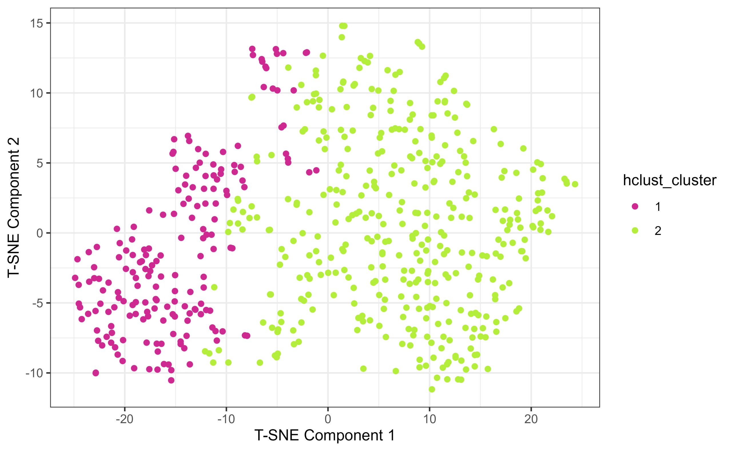
(9) Compare the Hierarchical Clustering to Diagnosis Labels with Dimensionality Reduction
Another way to interrogate how well clustering assigned clusters based on diagnosis label is to annotate the T-SNE plot you constructed earlier but this time instead of colouring the points by their known diagnosis label, you can annotate by their hierarchically-defined clusters.
Use the same perplexity and random seed as before.This way you can compare how the hclust clusters map on to the high dimensional space against how the diagnostic labels map onto the same space. When comparing tsne maps annotated by diagnosis, and by hclust cluster, what do you notice? What similarities and differences stand out to you?
## --------------------------------------------------- ##
##### Repeat T-SNE code but plot coloured by hclust #####
## --------------------------------------------------- ##
# Set your perplexity and seed
set.seed (789)
perplexity <- 30
seed <- 789

# Perform t-SNE with the specified perplexity and seed
tsne_model <- Rtsne(Diagnostic.Features.Scored, perplexity = perplexity, seed = seed)

# Create a dataframe for the t-SNE components
tsne_data <- data.frame(
  tSNE1 = tsne_model$Y[, 1],
  tSNE2 = tsne_model$Y[, 2],
  hclust_cluster = as.factor(All.Samples.zscored$hclust_clusters)  # Add the Hierarchical Cluster Assignment - convert to factor to make the scale discrete
)
view( tsne_data)
# Load ggplot2
library(ggplot2)
# specify the colour palette :
hclust.colours <- c("maroon3", "olivedrab2")

# Create the plot
tsne.by.hcluster <- ggplot(tsne_data, aes(x = tSNE1, y = tSNE2, colour = hclust_cluster)) +
  geom_point() +
  labs( x = "T-SNE Component 1", y= "T-SNE Component 2") +
  theme_bw() +
  scale_color_manual(values = hclust.colours)

# Print the plot
print(tsne.by.hcluster)
(10) Some final food for thought
(something for students to think about – can be made into a discussion about clustering algorithms, and why it’s important to verify and validate clustering outputs)
You compared the true diagnostic labels for breast cancer cells – benign and malignant to hierarchical clusters constructed solely from size and shape features. Based on how well the clustering algorithm separated benign and malignant cells, think about how useful this approach would have been if you did not know a priori that the cells were classified into benign and malignant diagnostic categories. After you clustered them into two groups and compared their statistics, what would you need to do to confirm the cells of one cluster being malignant and the others are benign?
