Sevda Montakhaby Nodeh
Early Childhood Development Lab
You are a researcher at the Early Childhood Development Research Center. Your latest project investigates how infants respond to different combinations of face race and music emotion. In specific you are interested in whether infants associate own- and other-race faces with music of different emotional valences (happy and sad music).
Your project was completed in collaboration with your colleagues in China. While you were responsible for designing your experiment, your collaborators were responsible for recruiting participants and collecting your data.
Chinese infants (3 to 9 months old) were recruited to participate in your experiment. Each infant was randomly assigned to one of the four face-race + music conditions where they saw a series of neutral own- or other-race faces paired with happy or sad musical excerpts.
- Own-race + happy-music condition (own-happy)
- Own-race + sad-music (own-sad)
- Other-race + happy music (other-happy)
- Other-race + sad music (other-sad)
In the own-happy, infants watched six Asian face videos sequentially paired with six happy musical excerpts. In other-sad, infants watched six African face videos sequentially paired with happy musical excerpts. In general, conditions were procedurally the same, except for the face-music composition. Infant eye movements were recorded using an eye tracker.
Your goal is to determine how face race and music emotion, as well as their interaction, influence the looking behaviour of infants.
Your independent variables:
- Face.Race(Chinese/African)
- Music.Emotion(Happy/Sad)
Your dependent variables:
- First.Face.Looking.Time: this is the looking time on the first face video in all four conditions
- Total.Looking.Time: Summ of each infant’s looking times to the subsequent five faces to create a measure of their total looking time to the five faces after.
Let’s begin by loading the required libraries and the dataset as “BabyData”. To do so download the file “infant_eye_tracking_study.csv” and run the following code. Remember to replace ‘path_to_your_downloaded_file’ with the actual path to the dataset on your system.
Note: Shaded boxes hold the R code, with the “#” sign indicating a comment that won’t execute in RStudio.
BabyData <- read.csv('path_to_your_downloaded_file/infant_eye_tracking_study.csv')
library(rstatix) #for performing basic statistical tests
library(dplyr) #for sorting data
library(tidyr) #for data sorting and structure
library(ggplot2) #for visualizing your data
library(readr)
library(ggpubr)
library(gridExtra)
Files to Download:
Please complete the accompanying exercises to the best of your abilities.
Answer Key
Exercise 1: Data Preparation and Exploration
Note: Shaded boxes hold the R code, while the white boxes display the code’s output, just as it appears in RStudio.
The “#” sign indicates a comment that won’t execute in RStudio.
1. Display the first few rows to understand your dataset.
summary(BabyData) # Viewing the summary of the dataset to check for inconsistencies
## Age.in.Days Condition Face.Race Music.Emotion Age.Group
## 1 93 Other-Race Happy Music African happy 3
## 2 98 Other-Race Happy Music African happy 3
## 3 93 Other-Race Happy Music African happy 3
## 4 93 Other-Race Happy Music African happy 3
## 5 93 Other-Race Happy Music African happy 3
## 6 100 Other-Race Happy Music African happy 3
## Total.Looking.Time First.Face.Looking.Time Participant.ID
## 1 44.035 8.273 HJOGM7704U
## 2 18.324 6.938 JHSEG5414N
## 3 24.600 4.225 OCQFX4970K
## 4 12.919 7.537 KLDOF5559R
## 5 12.755 4.230 HHPGJ9661Y
## 6 38.777 9.351 NVCPX9518V
2. Use relocate() to re-order your columns such that your “Participant.ID” column appears as the first column in your dataset.
BabyData <- BabyData %>% relocate(Participant.ID, .before = Age.in.Days)
3. Check your data for any missing values. Remove any rows with missing or NA values from the dataset.
sum(is.na(BabyData)) # Checking for missing values in the dataset
## [1] 3
BabyData <- BabyData[!is.na(BabyData$First.Face.Looking.Time), ]
## Participant.ID Age.in.Days Condition Face.Race
## Length:193 Min. : 79.0 Length:193 Length:193
## Class :character 1st Qu.:127.0 Class :character Class :character
## Mode :character Median :185.0 Mode :character Mode :character
## Mean :189.3
## 3rd Qu.:246.0
## Max. :316.0
##
## Music.Emotion Age.Group Total.Looking.Time First.Face.Looking.Time
## Length:193 Min. :3.000 Min. : 1.654 Min. : 0.160
## Class :character 1st Qu.:3.000 1st Qu.:20.671 1st Qu.: 5.309
## Mode :character Median :6.000 Median :30.381 Median : 7.495
## Mean :6.093 Mean :29.196 Mean : 7.041
## 3rd Qu.:9.000 3rd Qu.:38.196 3rd Qu.: 9.185
## Max. :9.000 Max. :50.000 Max. :11.823
## NA's :3
4. Check your data again for any missing values and check data consistency.
sum(is.na(BabyData)) # Checking for missing values in the dataset
## [1] 0
summary(BabyData) # Viewing the summary of the dataset to check for inconsistencies
## Participant.ID Age.in.Days Condition Face.Race
## Length:193 Min. : 79.0 Length:193 Length:193
## Class :character 1st Qu.:127.0 Class :character Class :character
## Mode :character Median :185.0 Mode :character Mode :character
## Mean :189.3
## 3rd Qu.:246.0
## Max. :316.0
##
## Music.Emotion Age.Group Total.Looking.Time First.Face.Looking.Time
## Length:193 Min. :3.000 Min. : 1.654 Min. : 0.160
## Class :character 1st Qu.:3.000 1st Qu.:20.671 1st Qu.: 5.309
## Mode :character Median :6.000 Median :30.381 Median : 7.495
## Mean :6.093 Mean :29.196 Mean : 7.041
## 3rd Qu.:9.000 3rd Qu.:38.196 3rd Qu.: 9.185
## Max. :9.000 Max. :50.000 Max. :11.823
## NA's :0
5. Check for structure and ensure that your factor columns (Music.Emotion, Face.Race, and Condition) are set-up correctly.
str(BabyData)
## 'data.frame': 190 obs. of 8 variables:
## $ Participant.ID : chr "HJOGM7704U" "JHSEG5414N" "OCQFX4970K" "KLDOF5559R" ...
## $ Age.in.Days : int 93 98 93 93 93 100 93 91 98 100 ...
## $ Condition : chr "Other-Race Happy Music" "Other-Race Happy Music" "Other-Race Happy Music" "Other-Race Happy Music" ...
## $ Face.Race : chr "African" "African" "African" "African" ...
## $ Music.Emotion : chr "happy" "happy" "happy" "happy" ...
## $ Age.Group : int 3 3 3 3 3 3 3 3 3 3 ...
## $ Total.Looking.Time : num 44 18.3 24.6 12.9 12.8 ...
## $ First.Face.Looking.Time: num 8.27 6.94 4.22 7.54 4.23 ...
BabyData$Face.Race <- as.factor(BabyData$Face.Race)
BabyData$Music.Emotion <- as.factor(BabyData$Music.Emotion)
BabyData$Condition <- as.factor(BabyData$Condition)
6. Check to see if your design is balanced or unbalanced.
table(BabyData$Age.Group, BabyData$Condition) #unbalanced design
##
## Other-Race Happy Music Other-Race Sad Music Own-Race Happy Music
## 3 16 12 12
## 6 15 19 19
## 9 14 17 17
##
## Own-Race Sad Music
## 3 17
## 6 15
## 9 17
Exercise 2: Conducting a Multi-Variable Linear Regression Analysis
7. Conduct a multi-variable linear regression on the first face looking time as the predicted variable, with Group, face race, and their interactions as the predictors. Display the result.
lm_model1 <- lm(First.Face.Looking.Time ~ Age.Group*Face.Race, data = BabyData)
summary(lm_model1)
##
## Call:
## lm(formula = First.Face.Looking.Time ~ Age.Group * Face.Race,
## data = BabyData)
##
## Residuals:
## Min 1Q Median 3Q Max
## -7.4524 -1.4478 0.3645 2.0507 4.5670
##
## Coefficients:
## Estimate Std. Error t value Pr(>|t|)
## (Intercept) 5.50710 0.75573 7.287 8.75e-12 ***
## Age.Group 0.22815 0.11542 1.977 0.0496 *
## Face.RaceChinese -0.04233 1.05722 -0.040 0.9681
## Age.Group:Face.RaceChinese 0.05036 0.16071 0.313 0.7544
## ---
## Signif. codes: 0 '***' 0.001 '**' 0.01 '*' 0.05 '.' 0.1 ' ' 1
##
## Residual standard error: 2.658 on 186 degrees of freedom
## Multiple R-squared: 0.05411, Adjusted R-squared: 0.03885
## F-statistic: 3.546 on 3 and 186 DF, p-value: 0.01564
8. Conduct a multivariable linear regression similar to the one described in the previous question. You predicted variable should be Total looking time, with Age.Group, Face.Race, Musical.Emotion, and their interactions as the predictors.
lm_model2 <- model <- lm(Total.Looking.Time ~ Age.Group * Face.Race * Music.Emotion, data = BabyData)
summary(lm_model2)
##
## Call:
## lm(formula = Total.Looking.Time ~ Age.Group * Face.Race * Music.Emotion,
## data = BabyData)
##
## Residuals:
## Min 1Q Median 3Q Max
## -24.8431 -8.0316 -0.1786 8.2809 27.7472
##
## Coefficients:
## Estimate Std. Error t value
## (Intercept) 28.0472 4.5406 6.177
## Age.Group -0.5167 0.7144 -0.723
## Face.RaceChinese -11.5424 6.6960 -1.724
## Music.Emotionsad -15.2955 6.6960 -2.284
## Age.Group:Face.RaceChinese 3.0376 1.0229 2.970
## Age.Group:Music.Emotionsad 3.4057 1.0229 3.330
## Face.RaceChinese:Music.Emotionsad 26.8342 9.3820 2.860
## Age.Group:Face.RaceChinese:Music.Emotionsad -5.7421 1.4252 -4.029
## Pr(>|t|)
## (Intercept) 4.16e-09 ***
## Age.Group 0.47045
## Face.RaceChinese 0.08645 .
## Music.Emotionsad 0.02351 *
## Age.Group:Face.RaceChinese 0.00338 **
## Age.Group:Music.Emotionsad 0.00105 **
## Face.RaceChinese:Music.Emotionsad 0.00473 **
## Age.Group:Face.RaceChinese:Music.Emotionsad 8.22e-05 ***
## ---
## Signif. codes: 0 '***' 0.001 '**' 0.01 '*' 0.05 '.' 0.1 ' ' 1
##
## Residual standard error: 11.72 on 182 degrees of freedom
## Multiple R-squared: 0.1742, Adjusted R-squared: 0.1425
## F-statistic: 5.486 on 7 and 182 DF, p-value: 9.76e-06
9. Given the significant three-way interaction, conduct Pearson correlation analyses to examine the linear relationship between total face looking time and participant age in days in each condition.
- (a) Begin by identifying all the unique conditions present in the dataset.
- (b) Performs a Pearson correlation analysis between Age group and Total Looking Time for each unique condition.
- (c) Stores and prints the correlation results, including correlation coefficients and p-values, for each condition.
unique_conditions <- unique(BabyData$Condition) #Get unique conditions
correlation_results <- list() ## Initialize a list to store results
# Loop through each condition and perform Pearson correlation
for (condition in unique_conditions) {
# Subset data for the current condition
subset_data <- subset(BabyData, Condition == condition)
subset_data$Age.Group <- as.numeric(as.character(subset_data$Age.Group))
# Perform Pearson correlation
correlation_test <- cor.test(subset_data$Age.Group, subset_data$Total.Looking.Time, method = "pearson")
# Store the result
correlation_results[[condition]] <- correlation_test
}
# Print the results
correlation_results
## $`Other-Race Happy Music`
##
## Pearson's product-moment correlation
##
## data: subset_data$Age.Group and subset_data$Total.Looking.Time
## t = -0.64059, df = 43, p-value = 0.5252
## alternative hypothesis: true correlation is not equal to 0
## 95 percent confidence interval:
## -0.3799180 0.2020743
## sample estimates:
## cor
## -0.09722666
##
##
## $`Other-Race Sad Music`
##
## Pearson's product-moment correlation
##
## data: subset_data$Age.Group and subset_data$Total.Looking.Time
## t = 4.4535, df = 46, p-value = 5.356e-05
## alternative hypothesis: true correlation is not equal to 0
## 95 percent confidence interval:
## 0.3136678 0.7206311
## sample estimates:
## cor
## 0.5488839
##
##
## $`Own-Race Happy Music`
##
## Pearson's product-moment correlation
##
## data: subset_data$Age.Group and subset_data$Total.Looking.Time
## t = 3.8943, df = 46, p-value = 0.0003166
## alternative hypothesis: true correlation is not equal to 0
## 95 percent confidence interval:
## 0.2490419 0.6851408
## sample estimates:
## cor
## 0.4979416
##
##
## $`Own-Race Sad Music`
##
## Pearson's product-moment correlation
##
## data: subset_data$Age.Group and subset_data$Total.Looking.Time
## t = 0.25438, df = 47, p-value = 0.8003
## alternative hypothesis: true correlation is not equal to 0
## 95 percent confidence interval:
## -0.2466891 0.3149919
## sample estimates:
## cor
## 0.03707966
Exercise 3: Visualizing Your Data
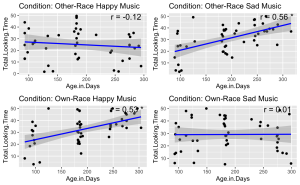
10. Visualize the relationship between total face looking time and participant age in days, categorized by different experimental conditions. Each condition should be represented in its own panel within a single figure. Additionally, for each panel:
- (a) Plot each infant’s total face looking time as a function of their age in days.
- (b) Add a blue linear regression line to indicate the trend.
- (c) Display the Pearson correlation coefficient you calculated in the previous question in the upper-right corner of each panel. Round your calculations for display to two decimal places.
- (d) Use different panels for each experimental condition and arrange them in a grid layout.
- (e) Ensure that a significant correlation (p < .05) is indicated with an asterisk.
# Get unique conditions
conditions <- unique(BabyData$Condition)
# Create a list to store plots
plot_list <- list()
# Loop through each condition and create a plot
for (condition in conditions) {
# Subset data for the condition
subset_data <- subset(BabyData, Condition == condition)
# Perform linear regression
fit <- lm(Total.Looking.Time ~ Age.in.Days, data = subset_data)
# Calculate Pearson correlation
cor_test <- cor.test(subset_data$Age.in.Days, subset_data$Total.Looking.Time)
# Create a scatter plot with regression line
p <- ggplot(subset_data, aes(x = Age.in.Days, y = Total.Looking.Time)) +
geom_point() +
geom_smooth(method = 'lm', color = 'blue') +
ggtitle(paste('Condition:', condition)) +
annotate("text", x = Inf, y = Inf, label = paste('r =', round(cor_test$estimate, 2), ifelse(cor_test$p.value < 0.05, "*", "")),
hjust = 1.1, vjust = 1.1, size = 5)
# Add plot to list
plot_list[[condition]] <- p
}
do.call(grid.arrange, c(plot_list, ncol = 2))
Exercise 4: Conducting Independent Sample T-tests
11. Analyze the impact of music emotional valence on the looking time for own- and other-race faces among different infant age groups (3, 6, and 9 months). Specifically, you are required to perform a series of independent sample t-tests.
- (a) Using the Age.Group column, conduct independent sample t-tests to examine the effects of music emotional valence (Music. Emotion) on the looking time (Total.Looking.Time) for own- and other-race faces (Face.Race) in each age group.
- (b) Ensure your script accounts for different combinations of age groups and music emotional valences.
- (c) Store and display the results of these t-tests in an organized manner.
# Ensure Age.Group is treated as a factor
BabyData$Age.Group <- as.factor(BabyData$Age.Group)
# Perform t-tests for each combination of Age.Group, Music.Emotion, and Face.Race
results <- list()
for(age_group in levels(BabyData$Age.Group)) {
for(music_emotion in unique(BabyData$Music.Emotion)) {
# Filter data for specific age group and music emotion
subset_data <- BabyData %>%
filter(Age.Group == age_group, Music.Emotion == music_emotion)
# Perform the t-test comparing Total.Looking.Time for own- vs. other-race faces
t_test_result <- t.test(Total.Looking.Time ~ Face.Race, data = subset_data)
# Store the results
result_name <- paste(age_group, music_emotion, sep="_")
results[[result_name]] <- t_test_result
}
}
# Print results
print(results)
## $`3_happy`
##
## Welch Two Sample t-test
##
## data: Total.Looking.Time by Face.Race
## t = -0.3153, df = 22.294, p-value = 0.7555
## alternative hypothesis: true difference in means between group African and group Chinese is not equal to 0
## 95 percent confidence interval:
## -12.465591 9.173257
## sample estimates:
## mean in group African mean in group Chinese
## 22.76875 24.41492
##
##
## $`3_sad`
##
## Welch Two Sample t-test
##
## data: Total.Looking.Time by Face.Race
## t = -1.0492, df = 22.86, p-value = 0.3051
## alternative hypothesis: true difference in means between group African and group Chinese is not equal to 0
## 95 percent confidence interval:
## -17.297369 5.658457
## sample estimates:
## mean in group African mean in group Chinese
## 21.32725 27.14671
##
##
## $`6_happy`
##
## Welch Two Sample t-test
##
## data: Total.Looking.Time by Face.Race
## t = 0.43226, df = 27.324, p-value = 0.6689
## alternative hypothesis: true difference in means between group African and group Chinese is not equal to 0
## 95 percent confidence interval:
## -6.401791 9.821475
## sample estimates:
## mean in group African mean in group Chinese
## 32.90100 31.19116
##
##
## $`6_sad`
##
## Welch Two Sample t-test
##
## data: Total.Looking.Time by Face.Race
## t = -0.62019, df = 27.075, p-value = 0.5403
## alternative hypothesis: true difference in means between group African and group Chinese is not equal to 0
## 95 percent confidence interval:
## -9.635393 5.162123
## sample estimates:
## mean in group African mean in group Chinese
## 30.20163 32.43827
##
##
## $`9_happy`
##
## Welch Two Sample t-test
##
## data: Total.Looking.Time by Face.Race
## t = -6.0414, df = 21.29, p-value = 5.08e-06
## alternative hypothesis: true difference in means between group African and group Chinese is not equal to 0
## 95 percent confidence interval:
## -27.28467 -13.31931
## sample estimates:
## mean in group African mean in group Chinese
## 19.13607 39.43806
##
##
## $`9_sad`
##
## Welch Two Sample t-test
##
## data: Total.Looking.Time by Face.Race
## t = 3.0179, df = 26.642, p-value = 0.005546
## alternative hypothesis: true difference in means between group African and group Chinese is not equal to 0
## 95 percent confidence interval:
## 3.335708 17.533234
## sample estimates:
## mean in group African mean in group Chinese
## 38.68853 28.25406
Exercise 5 Creating a Bar Plots
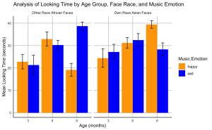
12. Create a bar plot to visualize the effects of music emotional valence on the looking time of infants at different ages for own- and other-race faces.
- (a) The plot should display the mean total looking time on the own- and other-race faces paired with happy or sad music for each age group.
- (b) Include standard error bars in your plot.
- (c) Organize the bars such that bars representing own-race faces are grouped together and labelled “Own Race Asian Faces”, followed by bars for other-race faces grouped together and labelled “Other Race African Faces”.
- (d) The colour of the bars should represent the music emotion: use blue for sad music and orange for happy music.
- (e) Label the x-axis as “Age (months)” and the y-axis as “Mean Looking Time (seconds)”.
- (f) Set the title of your plot as “Analysis of Looking Time by Age Group, Face Race, and Music Emotion”
- (g) Set the theme of your plot to minimal. Make sure the x- and y-axis lines are solid black lines.
- (h)Your plot should not display minor grid lines, major grid lines only.
# Calculate means and standard errors
data_summary <- BabyData %>%
group_by(Age.Group, Face.Race, Music.Emotion) %>%
summarize(Mean = mean(Total.Looking.Time),
SE = sd(Total.Looking.Time)/sqrt(n())) %>%
ungroup()
## `summarise()` has grouped output by 'Age.Group', 'Face.Race'. You can override
## using the `.groups` argument.
# Create the bar plot
ggplot(data_summary, aes(x = factor(Age.Group), y = Mean, fill = Music.Emotion)) +
geom_bar(stat = "identity", position = position_dodge()) +
geom_errorbar(aes(ymin = Mean - SE, ymax = Mean + SE),
position = position_dodge(0.9), width = 0.25) +
scale_fill_manual(values = c("happy" = "orange", "sad" = "blue")) +
facet_wrap(~ Face.Race, scales = "free_x", labeller = labeller(Face.Race = c(Chinese = "Own Race Asian Faces", African = "Other Race African Faces"))) +
labs(x = "Age (months)", y = "Mean Looking Time (seconds)", title = "Analysis of Looking Time by Age Group, Face Race, and Music Emotion") +
theme_minimal() +
theme(
panel.grid.minor = element_blank(),
panel.grid.major = element_line(color = "gray", size = 0.5, linetype = "solid"), # Major grid lines
axis.line = element_line(color = "black", size = 0.5) # Axis lines
)