Perception and Sensorimotor Lab

Welcome to the Perception and Sensorimotor Lab at McMaster University. As a budding cognitive psychologist here, you are about to embark on an explorative journey into the depth effect—a captivating psychological phenomenon that suggests visual events occurring in closer proximity (near space) are processed more efficiently than those farther away (far space). This effect provides a unique window into the cognitive architecture underpinning our sensory experiences, possibly implicating the involvement of the dorsal visual stream, which processes spatial relationships and movements in near space, and the ventral stream, known for its role in recognizing detailed visual information.

Your goal is to dissect whether the depth effect is task-dependent, aligning strictly with the dorsal/ventral stream dichotomy, or whether it represents a universal processing advantage for stimuli in near space across various cognitive tasks.

Your research journey begins in your lab. Imagine the lab as a gateway to a three-dimensional world, where the concept of depth is not only a subject of study but also a lived sensory experience for your participants! Seated inside a darkened tent, each participant grips a steering wheel, their primary tool for interaction and inputting responses. Before them, a screen comes to life with a 3D virtual environment meticulously engineered to test the frontiers of depth perception.

The virtual landscape participants encounter is a model of simplicity and complexity; as illustrated in the figure below, before the participants a ground plane extends into the depth of the screen, intersected by two sets of upright placeholder walls at varying depths—near and far. The walls stand on either side of the central axis, mirrored perfectly across the midline. The textures of the ground and placeholders—a random dot matrix and a checkerboard pattern, respectively—maintain a consistent density. These visual hints, alongside the textural gradients and the retinal size variance between near and far objects, act as subtle cues for depth perception.

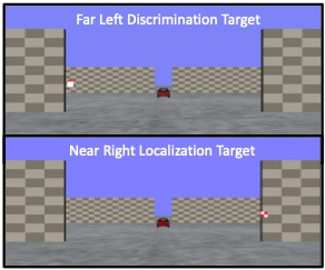
From their first-person point of view, participants are asked to:

1. Either discriminate the orientation of a red triangular target or localize a checkered square within this 3D dimensional immersive environment.
2. The targets could appear in both near and far spaces, demanding keen sensory discrimination and localization.

Through this experiment, you are not just observing the depth effect; you are dissecting it, unearthing the cognitive processes that allow humans to navigate the intricate dance of depth in our daily lives!

Let’s begin by loading the required libraries and the dataset. To do so download the file “NearFarRep_Outlier.csv” and run the following code.

Note: Shaded boxes hold the R code, with the “#” sign indicating a comment that won’t execute in RStudio.

Read in the downloaded dataset “NearFarRep_Outlier.csv” as “NearFarData”. Remember to replace ‘path_to_your_downloaded_file’ with the actual path to the dataset on your system.

The dataset contains the response times of participants and includes the following columns:

1. “Response” indicates the type of task (Discrimination or Localization)
2. “Con” indicating the target depth (Near or Far)
3. “TarRT” represents the target response times.

Files to Download:

1. NearFarRep_Outlier.csv

Please complete the accompanying exercises to the best of your abilities.

Answer Key

Exercise 1: Data Preparation and Exploration

Note: Shaded boxes hold the R code, while the white boxes display the code’s output, just as it appears in RStudio.
The “#” sign indicates a comment that won’t execute in RStudio. 

1. Display the first few rows to understand your dataset. Display all column names in the dataset.

2. Set up “Response” and “Con” as factors, then check the structure of your data to make sure your factors and levels are set up correctly.

3. Perform basic data checks for missing values and data consistency.

4. Convert the values in your dependent measures column “TarRT” to seconds.

Exercise 2: Visualizing Your Data

5. Using the “dplyr” package, write R code to calculate the mean response time and the standard error of the mean (SERT) for each combination of your two factors (Response and Con).
   # Calculate means and standard errors for each combination of 'Response' and 'Con'
summary_df <- NearFarData %>%
  group_by(Response, Con) %>%
  summarise(
    MeanRT = mean(TarRT),
    SERT = sd(TarRT) / sqrt(n())
  )

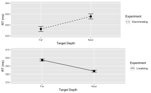
6. Using the “ggplot2” package, create a line plot with error bars for the Discrimination task.

• (a) The x-axis should represent the target depth (Con), and be labelled “Target Depth”.
• (b) The y-axis should represent the mean response time (MeanRT), and be labelled “RT (ms)”
• (c) Error bars should represent the standard error of the mean (SERT).
• (d) Ensure the line type is solid.
• (e) Set the minimum value of your y-axis to 630 and the maximum to 660.

7. Similarly, create a line plot with error bars for the Localization task. Use a dashed line for this plot with the following exceptions:

• (a) Ensure the line type is dashed
• (b) Set the minimum value of your y-axis to 370 and the maximum to 410.

Exercise 3: ANOVA Analysis

9. Using the “anova_test” function, conduct a two-way between-subjects ANOVA to investigate the effects of Con (Condition) and Response (Task type) on the target response times (TarRT). After running the ANOVA, use the “get_anova_table” function to present the results.

Exercise 4: Post Hoc Analysis

10. Use “lm” function to fit a linear model to your data. Make sure to specify your dependent variable, independent variables, and interaction terms.
    ## Fitting a linear model to data
lm_model <- lm(TarRT ~ Con * Response, data = NearFarData)

11. Use the “emmeans” function to get the estimated marginal means for your factors and their interaction. Then, use the pairs function to perform pairwise comparisons.
    • (a) Set the adjust parameter in the test function to “Tukey” for Tukey’s honest significant difference test, to adjust for multiple comparisons to control the family-wise error rate.

    # Get the estimated marginal means
emm <- emmeans(lm_model, specs = pairwise ~ Con * Response)