EdCog Lab

You are a researcher in the EdCog Lab at McMaster University. The Lab is conducting a study aimed at understanding the beliefs of instructors about student abilities in STEM (Science, Technology, Engineering, and Math) disciplines. This study is motivated by a growing body of literature suggesting that instructors’ beliefs about intelligence and success—categorized into brilliance belief (the idea that success requires innate talent), universality belief (the belief that success is achievable by everyone versus only a select few), and mindset beliefs (the view that intelligence and skills are either fixed or can change over time)—play a crucial role in educational practices and student outcomes. Understanding these beliefs is particularly important in STEM fields, where perceptions of innate talent versus learned skills can significantly influence teaching approaches and student engagement.

Experimental Design:

The survey was distributed through LimeSurvey to instructors across the Science, Health Sciences, and Engineering faculties. Participants were asked a series of Likert-scale questions (ranging from strongly disagree to strongly agree) aimed at assessing their beliefs in each of the three areas. Additional demographic and background questions were included to control for variables such as years of teaching experience, field of specialization, and level of education.

1. Brilliance Belief: The belief that only those with raw, innate talent can achieve success in their field.
2. Universality Belief: The belief that success is achievable for everyone, assuming the right effort and strategies are employed.
3. Mindset Beliefs: Instructors’ views on the nature of intelligence and skills—whether they are fixed traits or can be developed over time.

The sample data file (“EdCogData.xlsx) for this exercise is structured as such:

• ID: A unique identifier for each respondent.
• Brilliance1 to Brilliance5: Responses to statements measuring the belief in brilliance as a requirement for success.
  • A higher score in these columns indicates a belief that brilliance is a requirement for success.
• MindsetGrowth1 to MindsetGrowth5: Responses to questions aimed at assessing the belief in a growth mindset, suggesting that intelligence and abilities can develop over time.
  • A higher score in these columns indicates a strong growth mindset.
• Nonuniversality1 to Nonuniversality5:  Responses to statements measuring beliefs counter to universality, meaning that not everyone can succeed (i.e., success is not universal).
  • A higher score in these columns indicates a non-universal mindset to success.
• Universality1 to Universality5: Responses to statements measuring the belief in universality, or the idea that success is achievable by anyone with sufficient effort.
  • A higher score in these columns indicates a belief that with enough effort success is achievable (i.e., success is universal)
• MindsetFixed1 to MindsetFixed5: Responses to questions aimed at assessing the belief in a fixed mindset regarding intelligence and abilities. A fixed mindset believes that intelligence, talents, and abilities are fixed traits. They think these traits are innate and cannot be significantly developed or improved through effort or education.
  • A higher score in these columns indicates a strong fixed mindset.

Getting Started: Loading Libraries, setting the working directory, and loading the dataset

Let’s begin by running the following code in RStudio to load the required libraries. Make sure to read through the comments embedded throughout the code to understand what each line of code is doing.

Note: Shaded boxes hold the R code, with the “#” sign indicating a comment that won’t execute in RStudio.

Make sure to have the required dataset (“EdCogData.xlsx“) for this exercise downloaded. Set the working directory of your current R session to the folder with the downloaded dataset. You may do this manually in R studio by clicking on the “Session” tab at the top of the screen, and then clicking on “Set Working Directory”.

If the downloaded dataset file and your R session are within the same file, you may choose the option of setting your working directory to the “source file location” (the location where your current R session is saved). If they are in different folders then click on “choose directory” option and browse for the location of the downloaded dataset.

You may also do this by running the following code:

Once you have set your working directory either manually or by code, in the Console below you will see the full directory of your folder as the output.

Read in the downloaded dataset as “edcogData” and complete the accompanying exercises to the best of your abilities.

Files to Download:

1. EdCogData.xlsx

Answer Key

Exercise 1: Data Preparation and Exploration

Note: Shaded boxes hold the R code, while the white boxes display the code’s output, just as it appears in RStudio. The “#” sign indicates a comment that won’t execute in RStudio. 

Load the dataset into RStudio and inspect its structure.

1. How many rows and columns are in the dataset?
2. What are the column names?

Exercise 2: Data Preprocessing

Prepare the data for analysis by ensuring it is in the correct format.

1. Are there any missing values in the dataset?

Exercise 3: Aggregating Scores

1. Create aggregate scores for each dimension (Brilliance, Fixed, Growth, Nonuniversal, Universal).

2. Create a new data frame named “edcog.agg.wide” that contains only the ID column and the aggregated score columns from “edcogData”.

3. Convert “edcog.agg.wide” from a wide to a long format named “edcog.agg.long”, with the following columns:

• ID
• Dimension (with values of Brilliance, Fixed, Growth, Universal, and Nonuniversal)
• AggregateScore

Exercise 4: Creating Plots

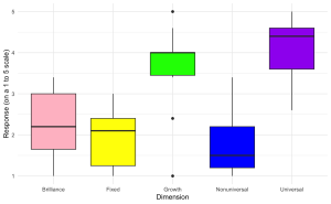
1. Create a boxplot to visualize the distribution of aggregate scores across different dimensions (Brilliance, Fixed, Growth, Nonuniversal, Universal) from the survey data with the following specifications:

• The x-axis should represent different ‘Dimensions’ of beliefs.
• The y-axis should represent the ‘Score’ on a scale from 1 to 5.
• Each ‘Dimension’ should have a different color fill for its box.
• Set the y-axis label to “Response (on a 1 to 5 scale)” and the x-axis label to “Dimension”.
• Use a minimal theme and remove the legend.
• Hint: Use “edcog.agg.long”

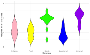
2. Generate a violin plot to visualize the distribution of aggregate scores for different dimensions (Brilliance, Fixed, Growth, Nonuniversal, Universal) from the survey data with the following specifications:

• The x-axis should represent different ‘Dimensions’ of beliefs.
• The y-axis should represent the ‘Score’ on a scale from 1 to 5.
• Each ‘Dimension’ should have a distinct color.
• Label the axes appropriately.
• Apply a minimalistic theme and consider removing the legend if it is not necessary.

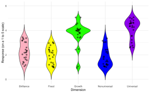
3. Enhance the violin plot by overlaying individual data points to show the raw data distribution alongside the aggregated density estimates.