Sevda Montakhaby Nodeh
Cognition and Memory Lab
Welcome! In this assignment, we will be entering a cognition and memory lab at McMaster University. Specifically, we will be examining data from an intriguing cognitive psychology study that explores the role of repetition in recognition memory.
Most of us are familiar with the phrase ‘practice makes perfect’. This motivational idiom aligns with intuition and is confirmed by many real-world observations. Much empirical research also supports this view–repeated opportunities to encode a stimulus improve subsequent memory retrieval and perceptual identification. These observations suggest that stimulus repetition strengthens underlying memory representations.
The present study focuses on a contradictory idea, that stimulus repetition can weaken memory encoding. The experiment comprised of three stages: a study phase, a distractor phase, and a surprise recognition memory test.
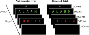
In the study phase participants aloud a red target word preceded by a briefly presented green prime word. On half of the trials, the prime and target were the same (repeated trials), and on the other half of the trials, the prime and target were different (not-repeated trials). In the figure below you can see an overview of the two different trial types. Following the study phase, participants engaged in a 10-minute distractor task consisting of math problems they had to solve by hand.
The final phase was a surprise recognition memory test where on each test trial they were shown a red word and asked to respond old if the word on the test was one they had previously seen at study, and new if they had never encountered the word before. Half of the trials at the test were words from the study phase and the other half were new words.
Let’s begin by running the following code to load the required libraries. Make sure to read through the comments embedded throughout the code to understand what each line of code is doing.
Note: Shaded boxes hold the R code, with the "#" sign indicating a comment that won't execute in RStudio.
# Load necessary libraries
library(rstatix) #for performing basic statistical tests
library(dplyr) #for sorting data
library(readxl) #for reading excel files
library(tidyr) #for data sorting and structure
library(ggplot2) #for visualizing your data
library(plotrix) #for computing basic summary stats
Make sure to have the required dataset (“RepDecrementdataset.xlsx”) for this exercise downloaded. Set the working directory of your current R session to the folder with the downloaded dataset. You may do this manually in R studio by clicking on the “Session” tab at the top of the screen, and then clicking on “Set Working Directory”.
If the downloaded dataset file and your R session are within the same file, you may choose the option of setting your working directory to the “source file location” (the location where your current R session is saved). If they are in different folders then click on “choose directory” option and browse for the location of the downloaded dataset.
You may also do this by running the following code
setwd(file.choose())
Once you have set your working directory either manually or by code, in the Console below you will see the full directory of your folder as the output.
Read in the downloaded dataset as “MemoryData” and complete the accompanying exercises to the best of your abilities.
MemoryData <- read_excel('RepDecrementdataset.xlsx')
Files to Download:
Answer Key
Exercise 1: Data Preparation and Exploration
Note: Shaded boxes hold the R code, while the white boxes display the code's output, just as it appears in RStudio.
The "#" sign indicates a comment that won't execute in RStudio.
1. Display the first few rows of your dataset to familiarize yourself with its structure and contents.
head(MemoryData) #Displaying the first few rows
## # A tibble: 6 × 7
## ID Hits_NRep Hits_Rep FalseAlarms Misses_Nrep Misses_Rep CorrectRej
## <dbl> <dbl> <dbl> <dbl> <dbl> <dbl> <dbl>
## 1 1 46 34 13 14 26 107
## 2 2 43 44 27 17 16 93
## 3 3 43 35 23 17 24 97
## 4 4 37 36 56 23 24 64
## 5 5 39 35 49 21 25 71
## 6 6 38 43 28 22 17 92
str(MemoryData) #Checking structure of dataset
## tibble [24 × 7] (S3: tbl_df/tbl/data.frame)
## $ ID : num [1:24] 1 2 3 4 5 6 7 8 9 10 ...
## $ Hits_NRep : num [1:24] 46 43 43 37 39 38 20 24 36 38 ...
## $ Hits_Rep : num [1:24] 34 44 35 36 35 43 11 29 43 27 ...
## $ FalseAlarms: num [1:24] 13 27 23 56 49 28 4 11 46 9 ...
## $ Misses_Nrep: num [1:24] 14 17 17 23 21 22 40 36 23 22 ...
## $ Misses_Rep : num [1:24] 26 16 24 24 25 17 49 31 17 33 ...
## $ CorrectRej : num [1:24] 107 93 97 64 71 92 116 109 74 111 ...
colnames(MemoryData)
## [1] "ID" "Hits_NRep" "Hits_Rep" "FalseAlarms" "Misses_Nrep"
## [6] "Misses_Rep" "CorrectRej"
2. Calculate Total Trials for Each Condition:
- (a) For each participant, sum the number of hits for non-repeated trials and missed non-repeated trials. Store this total in a new column named “TotalNRep”. The value should be 60 for all participants, reflecting the total number of non-repeated trial types.
- (b) Repeat the process for repeated trials, storing the sum in “TotalRep” (60 trials).
- (c) Similarly, sum the number of false alarms and correct rejections to represent the total number of new trials (120 trials) and store this in “TotalNew”.
Note that if the value in “TotalNRep” and “TotalRep” is less than 60 for a participant, it indicates that certain word trials were excluded during the study phase due to issues (e.g., the participant read aloud the prime word instead of the target, leading to trial spoilage).
MemoryData <- MemoryData %>%
mutate(TotalNRep = Hits_NRep + Misses_Nrep)
MemoryData <- MemoryData %>%
mutate(TotalRep = Hits_Rep + Misses_Rep)
MemoryData <- MemoryData %>%
mutate(TotalNew = FalseAlarms + CorrectRej)
3. Transform the counts in the hits, misses, false alarms, and correct rejections columns into proportions. Do this by dividing each count by the total number of trials for the respective condition (e.g., divide hits for non-repeated trials by “TotalNRep”).
MemoryData$Hits_NRep <- (MemoryData$Hits_NRep/MemoryData$TotalNRep)
MemoryData$Misses_Nrep <- (MemoryData$Misses_Nrep/MemoryData$TotalNRep)
MemoryData$Hits_Rep <- (MemoryData$Hits_Rep/MemoryData$TotalRep)
MemoryData$Misses_Rep <- (MemoryData$Misses_Rep/MemoryData$TotalRep)
MemoryData$CorrectRej <- (MemoryData$CorrectRej/MemoryData$TotalNew)
MemoryData$FalseAlarms <- (MemoryData$FalseAlarms/MemoryData$TotalNew)
4. Once the proportions are calculated, remove the “TotalNew”, “TotalRep”, and “TotalNRep” columns from the dataset as they are no longer needed for further analysis.
MemoryData <- MemoryData[, !names(MemoryData) %in% c("TotalNew", "TotalRep","TotalNRep")]
5. Use the pivot_longer() function from the tidyr package to convert your data from wide to long format. Pivot the columns “Hits_NRep”, “Hits_Rep”, and “FalseAlarms”, setting the new column names to “Condition” and “Proportion” for the reshaped data.
long_df <- MemoryData %>%
pivot_longer(
cols = c(Hits_NRep, Hits_Rep, FalseAlarms),
names_to = "Condition",
values_to = "Proportion"
)
Exercise 2: Computing Summary Stats and Correcting for Within-Subjects Variability
6. Using your long formatted dataset, group your data by ID and calculate the per-subject mean and the grand mean of the Proportions column.
- (a) Adjust each individual’s score by subtracting their mean and adding the grand mean.
- (b) Calculate the mean and SEM of the adjusted scores for each condition.
- (c) Use the adjusted scores to calculate the within-subject SEM. d.Group the data by Condition and calculate the mean and SEM.
data_adjusted <- long_df %>%
group_by(ID) %>%
mutate(SubjectMean = mean(Proportion, na.rm = TRUE)) %>%
ungroup() %>%
mutate(GrandMean = mean(Proportion, na.rm = TRUE)) %>%
mutate(AdjustedScore = Proportion - SubjectMean + GrandMean)
# Calculate the mean and SEM of the adjusted scores
summary_df <- data_adjusted %>%
group_by(Condition) %>%
summarize(
AdjustedMean = mean(AdjustedScore, na.rm = TRUE),
AdjustedSEM = sd(AdjustedScore, na.rm = TRUE) / sqrt(n())
)
Exercise 3: Visualizing your data
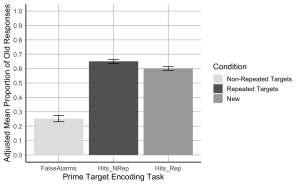
7. Create a bar plot where the x-axis represents the Prime-target Encoding task conditions, the y-axis shows the adjusted mean proportion of old responses, and include error bars represent the adjusted SEM. Begin by setting custom colours for each condition. The colour for the bar presenting the false alarms or “New” should be “gray89”; the colour for “Hits_Nrep” or “Non-Repeated Targets” bar should be “gray39”; the colour for the “Hits_Rep” or “Repeated Targets” bar should be “darkgrey”.
- (a) The x-axis should be titled “Prime Target Encoding Task”.
- (b) The y-axis should be titled “Adjusted Mean Proportion of Old Responses”
- (c) Add error bars to each bar to represent the corrected SEM.
- (d) Make the x and y-axis lines solid black.
- (e) Ensure the plot has a minimalistic design with major grid lines only.
- (f) Add a legend to indicate the Condition categories, the legend should read, Non-Repeated Targets instead of “Hits_Nrep”, Repeated Targets instead of “Hits_Rep”, and New instead of “False Alarms”.
- (g) Set the minimum and maximum values on your y-axis to 0 and 1, respectively.
- (h)The values on the y-axis should go up by 0.1
# Create the bar plot with adjusted SEM error bars
ggplot(summary_df, aes(x = Condition, y = AdjustedMean, fill = Condition)) +
geom_bar(stat = "identity", position = position_dodge()) +
geom_errorbar(aes(ymin = AdjustedMean - AdjustedSEM, ymax = AdjustedMean + AdjustedSEM), width = 0.2, position = position_dodge(0.9)) +
scale_fill_manual(values = c("Hits_NRep" = "gray39", "Hits_Rep" = "darkgrey", "FalseAlarms" = "gray89"),
labels = c("Non-Repeated Targets", "Repeated Targets", "New")) +
labs(
x = "Prime Target Encoding Task",
y = "Adjusted Mean Proportion of Old Responses",
fill = "Condition"
) +
scale_y_continuous(breaks = seq(0, 1, by = 0.1), limits = c(0, 1)) +
theme_minimal(base_size = 14) +
theme(
axis.line = element_line(color = "black"),
axis.title = element_text(color = "black"),
panel.grid.major = element_line(color = "grey", size = 0.5),
panel.grid.minor = element_blank(),
legend.title = element_text(color = "black")
)
Exercise 4: Computation
8. Using the wide formatted data file “MemoryData” conduct a two-paired sample t-test comparing the hit rate collapsed across the two repetition conditions (repeated/not-repeated) to the false alarm rate to assess participants’ ability to distinguish old from new items.
- (a) Calculate the mean hit rate by averaging the hit rates from the ‘Hits_NRep’ (non-repeated) and ‘Hits_Rep’ (repeated) conditions for each participant.
- (b) Conduct a paired sample t-test to compare the hit rate (collapsed across the two repetition conditions) to the false alarm rate to assess participants’ ability to distinguish old from new items.
collapsed_hitdata <- MemoryData %>%
mutate(HitRate = (Hits_NRep + Hits_Rep) / 2)
# Conduct paired sample t-tests
t_test_results <- t.test(collapsed_hitdata$HitRate, collapsed_hitdata$FalseAlarms, paired = TRUE)
print(t_test_results)
##
## Paired t-test
##
## data: collapsed_hitdata$HitRate and collapsed_hitdata$FalseAlarms
## t = 11.621, df = 23, p-value = 4.179e-11
## alternative hypothesis: true mean difference is not equal to 0
## 95 percent confidence interval:
## 0.3071651 0.4401983
## sample estimates:
## mean difference
## 0.3736817
#Hit rates were higher than false alarm rates, t(23) = 11.62, p < .001.
9. Using the wide formatted data file “MemoryData” conduct a two-paired sample t-test comparing the hit rates for the not-repeated and repeated targets.
# Conduct paired sample t-tests for non-repeated vs repeated hit rates
t_test_results_hits <- t.test(collapsed_hitdata$Hits_NRep, collapsed_hitdata$Hits_Rep, paired = TRUE)
# Print the results for the hit rate comparison
print(t_test_results_hits)
##
## Paired t-test
##
## data: collapsed_hitdata$Hits_NRep and collapsed_hitdata$Hits_Rep
## t = 2.5431, df = 23, p-value = 0.01817
## alternative hypothesis: true mean difference is not equal to 0
## 95 percent confidence interval:
## 0.009071364 0.088174399
## sample estimates:
## mean difference
## 0.04862288
#Hit rates were higher for not-repeated targets than for repeated targets, t(23) = 2.54, p = .018.
