58 Some Basic Null Hypothesis Tests
Learning Objectives
- Conduct and interpret one-sample, dependent-samples, and independent-samples t- tests.
- Interpret the results of one-way, repeated measures, and factorial ANOVAs.
- Conduct and interpret null hypothesis tests of Pearson’s r.
In this section, we look at several common null hypothesis testing procedures. The emphasis here is on providing enough information to allow you to conduct and interpret the most basic versions. In most cases, the online statistical analysis tools mentioned in Chapter 12 will handle the computations—as will programs such as Microsoft Excel and SPSS.
The t-Test
As we have seen throughout this book, many studies in psychology focus on the difference between two means. The most common null hypothesis test for this type of statistical relationship is the t- test. In this section, we look at three types of t tests that are used for slightly different research designs: the one-sample t-test, the dependent-samples t- test, and the independent-samples t- test. You may have already taken a course in statistics, but we will refresh your statistical
One-Sample t-Test
The one-sample t-test is used to compare a sample mean (M) with a hypothetical population mean (μ0) that provides some interesting standard of comparison. The null hypothesis is that the mean for the population (µ) is equal to the hypothetical population mean: μ = μ0. The alternative hypothesis is that the mean for the population is different from the hypothetical population mean: μ ≠ μ0. To decide between these two hypotheses, we need to find the probability of obtaining the sample mean (or one more extreme) if the null hypothesis were true. But finding this p value requires first computing a test statistic called t. (A test statistic is a statistic that is computed only to help find the p value.) The formula for t is as follows:
 Again, M is the sample mean and µ0 is the hypothetical population mean of interest. SD is the sample standard deviation and N is the sample size.
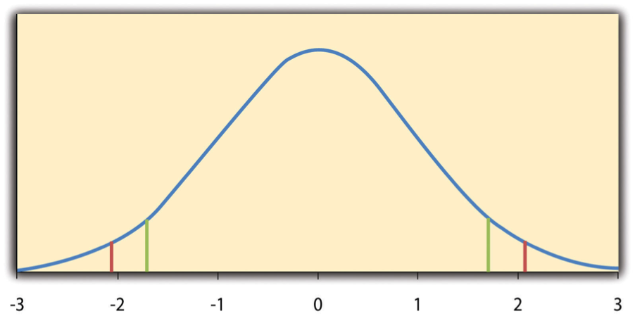
The reason the t statistic (or any test statistic) is useful is that we know how it is distributed when the null hypothesis is true. As shown in Figure 13.1, this distribution is unimodal and symmetrical, and it has a mean of 0. Its precise shape depends on a statistical concept called the degrees of freedom, which for a one-sample t-test is N − 1. (There are 24 degrees of freedom for the distribution shown in Figure 13.1.) The important point is that knowing this distribution makes it possible to find the p value for any t score. Consider, for example, a t score of 1.50 based on a sample of 25. The probability of a t score at least this extreme is given by the proportion of t scores in the distribution that are at least this extreme. For now, let us define extreme as being far from zero in either direction. Thus the p value is the proportion of t scores that are 1.50 or above or that are −1.50 or below—a value that turns out to be .14.
Fortunately, we do not have to deal directly with the distribution of t scores. If we were to enter our sample data and hypothetical mean of interest into one of the online statistical tools in Chapter 12 or into a program like SPSS (Excel does not have a one-sample t-test function), the output would include both the t score and the p value. At this point, the rest of the procedure is simple. If p is equal to or less than .05, we reject the null hypothesis and conclude that the population mean differs from the hypothetical mean of interest. If p is greater than .05, we retain the null hypothesis and conclude that there is not enough evidence to say that the population mean differs from the hypothetical mean of interest. (Again, technically, we conclude only that we do not have enough evidence to conclude that it does differ.)
If we were to compute the t score by hand, we could use a table like Table 13.2 to make the decision. This table does not provide actual p values. Instead, it provides the critical values of t for different degrees of freedom (df) when α is .05. For now, let us focus on the two-tailed critical values in the last column of the table. Each of these values should be interpreted as a pair of values: one positive and one negative. For example, the two-tailed critical values when there are 24 degrees of freedom are 2.064 and −2.064. These are represented by the red vertical lines in Figure 13.1. The idea is that any t score below the lower critical value (the left-hand red line in Figure 13.1) is in the lowest 2.5% of the distribution, while any t score above the upper critical value (the right-hand red line) is in the highest 2.5% of the distribution. Therefore any t score beyond the critical value in either direction is in the most extreme 5% of t scores when the null hypothesis is true and has a p value less than .05. Thus if the t score we compute is beyond the critical value in either direction, then we reject the null hypothesis. If the t score we compute is between the upper and lower critical values, then we retain the null hypothesis.
| Critical value | ||
| df | One-tailed | Two-tailed |
| 3 | 2.353 | 3.182 |
| 4 | 2.132 | 2.776 |
| 5 | 2.015 | 2.571 |
| 6 | 1.943 | 2.447 |
| 7 | 1.895 | 2.365 |
| 8 | 1.860 | 2.306 |
| 9 | 1.833 | 2.262 |
| 10 | 1.812 | 2.228 |
| 11 | 1.796 | 2.201 |
| 12 | 1.782 | 2.179 |
| 13 | 1.771 | 2.160 |
| 14 | 1.761 | 2.145 |
| 15 | 1.753 | 2.131 |
| 16 | 1.746 | 2.120 |
| 17 | 1.740 | 2.110 |
| 18 | 1.734 | 2.101 |
| 19 | 1.729 | 2.093 |
| 20 | 1.725 | 2.086 |
| 21 | 1.721 | 2.080 |
| 22 | 1.717 | 2.074 |
| 23 | 1.714 | 2.069 |
| 24 | 1.711 | 2.064 |
| 25 | 1.708 | 2.060 |
| 30 | 1.697 | 2.042 |
| 35 | 1.690 | 2.030 |
| 40 | 1.684 | 2.021 |
| 45 | 1.679 | 2.014 |
| 50 | 1.676 | 2.009 |
| 60 | 1.671 | 2.000 |
| 70 | 1.667 | 1.994 |
| 80 | 1.664 | 1.990 |
| 90 | 1.662 | 1.987 |
| 100 | 1.660 | 1.984 |
Thus far, we have considered what is called a two-tailed test, where we reject the null hypothesis if the t score for the sample is extreme in either direction. This test makes sense when we believe that the sample mean might differ from the hypothetical population mean but we do not have good reason to expect the difference to go in a particular direction. But it is also possible to do a one-tailed test, where we reject the null hypothesis only if the t score for the sample is extreme in one direction that we specify before collecting the data. This test makes sense when we have good reason to expect the sample mean will differ from the hypothetical population mean in a particular direction.
Here is how it works. Each one-tailed critical value in Table 13.2 can again be interpreted as a pair of values: one positive and one negative. A t score below the lower critical value is in the lowest 5% of the distribution, and a t score above the upper critical value is in the highest 5% of the distribution. For 24 degrees of freedom, these values are −1.711 and 1.711. (These are represented by the green vertical lines in Figure 13.1.) However, for a one-tailed test, we must decide before collecting data whether we expect the sample mean to be lower than the hypothetical population mean, in which case we would use only the lower critical value, or we expect the sample mean to be greater than the hypothetical population mean, in which case we would use only the upper critical value. Notice that we still reject the null hypothesis when the t score for our sample is in the most extreme 5% of the t scores we would expect if the null hypothesis were true—so α remains at .05. We have simply redefined extreme to refer only to one tail of the distribution. The advantage of the one-tailed test is that critical values are less extreme. If the sample mean differs from the hypothetical population mean in the expected direction, then we have a better chance of rejecting the null hypothesis. The disadvantage is that if the sample mean differs from the hypothetical population mean in the unexpected direction, then there is no chance at all of rejecting the null hypothesis.
Example One-Sample t–Test
Imagine that a health psychologist is interested in the accuracy of university students’ estimates of the number of calories in a chocolate chip cookie. He shows the cookie to a sample of 10 students and asks each one to estimate the number of calories in it. Because the actual number of calories in the cookie is 250, this is the hypothetical population mean of interest (µ0). The null hypothesis is that the mean estimate for the population (μ) is 250. Because he has no real sense of whether the students will underestimate or overestimate the number of calories, he decides to do a two-tailed test. Now imagine further that the participants’ actual estimates are as follows:
250, 280, 200, 150, 175, 200, 200, 220, 180, 250.
The mean estimate for the sample (M) is 212.00 calories and the standard deviation (SD) is 39.17. The health psychologist can now compute the t score for his sample:
 If he enters the data into one of the online analysis tools or uses SPSS, it would also tell him that the two-tailed p value for this t score (with 10 − 1 = 9 degrees of freedom) is .013. Because this is less than .05, the health psychologist would reject the null hypothesis and conclude that university students tend to underestimate the number of calories in a chocolate chip cookie. If he computes the t score by hand, he could look at Table 13.2 and see that the critical value of t for a two-tailed test with 9 degrees of freedom is ±2.262. The fact that his t score was more extreme than this critical value would tell him that his p value is less than .05 and that he should reject the null hypothesis. Using APA style, these results would be reported as follows: t(9) = -3.07, p = .01. Note that the t and p are italicized, the degrees of freedom appear in brackets with no decimal remainder, and the values of t and p are rounded to two decimal places.
Finally, if this researcher had gone into this study with good reason to expect that university students underestimate the number of calories, then he could have done a one-tailed test instead of a two-tailed test. The only thing this decision would change is the critical value, which would be −1.833. This slightly less extreme value would make it a bit easier to reject the null hypothesis. However, if it turned out that university students overestimate the number of calories—no matter how much they overestimate it—the researcher would not have been able to reject the null hypothesis.
The Dependent-Samples t–Test
The dependent-samples t-test (sometimes called the paired-samples t-test) is used to compare two means for the same sample tested at two different times or under two different conditions. This comparison is appropriate for pretest-posttest designs or within-subjects experiments. The null hypothesis is that the means at the two times or under the two conditions are the same in the population. The alternative hypothesis is that they are not the same. This test can also be one-tailed if the researcher has good reason to expect the difference goes in a particular direction.
It helps to think of the dependent-samples t-test as a special case of the one-sample t-test. However, the first step in the dependent-samples t-test is to reduce the two scores for each participant to a single difference score by taking the difference between them. At this point, the dependent-samples t-test becomes a one-sample t-test on the difference scores. The hypothetical population mean (µ0) of interest is 0 because this is what the mean difference score would be if there were no difference on average between the two times or two conditions. We can now think of the null hypothesis as being that the mean difference score in the population is 0 (µ0 = 0) and the alternative hypothesis as being that the mean difference score in the population is not 0 (µ0 ≠ 0).
Example Dependent-Samples t–Test
Imagine that the health psychologist now knows that people tend to underestimate the number of calories in junk food and has developed a short training program to improve their estimates. To test the effectiveness of this program, he conducts a pretest-posttest study in which 10 participants estimate the number of calories in a chocolate chip cookie before the training program and then again afterward. Because he expects the program to increase the participants’ estimates, he decides to do a one-tailed test. Now imagine further that the pretest estimates are
230, 250, 280, 175, 150, 200, 180, 210, 220, 190
and that the posttest estimates (for the same participants in the same order) are
250, 260, 250, 200, 160, 200, 200, 180, 230, 240.
The difference scores, then, are as follows:
20, 10, −30, 25, 10, 0, 20, −30, 10, 50.
Note that it does not matter whether the first set of scores is subtracted from the second or the second from the first as long as it is done the same way for all participants. In this example, it makes sense to subtract the pretest estimates from the posttest estimates so that positive difference scores mean that the estimates went up after the training and negative difference scores mean the estimates went down.
The mean of the difference scores is 8.50 with a standard deviation of 27.27. The health psychologist can now compute the t score for his sample as follows:
 If he enters the data into one of the online analysis tools or uses Excel or SPSS, it would tell him that the one-tailed p value for this t score (again with 10 − 1 = 9 degrees of freedom) is .148. Because this is greater than .05, he would retain the null hypothesis and conclude that the training program does not significantly increase people’s calorie estimates. If he were to compute the t score by hand, he could look at Table 13.2 and see that the critical value of t for a one-tailed test with 9 degrees of freedom is 1.833. (It is positive this time because he was expecting a positive mean difference score.) The fact that his t score was less extreme than this critical value would tell him that his p value is greater than .05 and that he should fail to reject the null hypothesis.
The Independent-Samples t-Test
The independent-samples t-test is used to compare the means of two separate samples (M1 and M2). The two samples might have been tested under different conditions in a between-subjects experiment, or they could be pre-existing groups in a cross-sectional design (e.g., women and men, extraverts and introverts). The null hypothesis is that the means of the two populations are the same: µ1 = µ2. The alternative hypothesis is that they are not the same: µ1 ≠ µ2. Again, the test can be one-tailed if the researcher has good reason to expect the difference goes in a particular direction.
The t statistic here is a bit more complicated because it must take into account two sample means, two standard deviations, and two sample sizes. The formula is as follows:
 Notice that this formula includes squared standard deviations (the variances) that appear inside the square root symbol. Also, lowercase n1 and n2 refer to the sample sizes in the two groups or condition (as opposed to capital N, which generally refers to the total sample size). The only additional thing to know here is that there are N − 2 degrees of freedom for the independent-samples t- test.
Example Independent-Samples t–Test
Now the health psychologist wants to compare the calorie estimates of people who regularly eat junk food with the estimates of people who rarely eat junk food. He believes the difference could come out in either direction so he decides to conduct a two-tailed test. He collects data from a sample of eight participants who eat junk food regularly and seven participants who rarely eat junk food. The data are as follows:
Junk food eaters: 180, 220, 150, 85, 200, 170, 150, 190
Non–junk food eaters: 200, 240, 190, 175, 200, 300, 240
The mean for the non-junk food eaters is 220.71 with a standard deviation of 41.23. The mean for the junk food eaters is 168.12 with a standard deviation of 42.66. He can now compute his t score as follows:
 If he enters the data into one of the online analysis tools or uses Excel or SPSS, it would tell him that the two-tailed p value for this t score (with 15 − 2 = 13 degrees of freedom) is .015. Because this p value is less than .05, the health psychologist would reject the null hypothesis and conclude that people who eat junk food regularly make lower calorie estimates than people who eat it rarely. If he were to compute the t score by hand, he could look at Table 13.2 and see that the critical value of t for a two-tailed test with 13 degrees of freedom is ±2.160. The fact that his t score was more extreme than this critical value would tell him that his p value is less than .05 and that he should reject the null hypothesis.
The Analysis of Variance
T-tests are used to compare two means (a sample mean with a population mean, the means of two conditions or two groups). When there are more than two groups or condition means to be compared, the most common null hypothesis test is the analysis of variance (ANOVA). In this section, we look primarily at the one-way ANOVA, which is used for between-subjects designs with a single independent variable. We then briefly consider some other versions of the ANOVA that are used for within-subjects and factorial research designs.
One-Way ANOVA
The one-way ANOVA is used to compare the means of more than two samples (M1, M2…MG) in a between-subjects design. The null hypothesis is that all the means are equal in the population: µ1= µ2 =…= µG. The alternative hypothesis is that not all the means in the population are equal.
The test statistic for the ANOVA is called F. It is a ratio of two estimates of the population variance based on the sample data. One estimate of the population variance is called the mean squares between groups (MSB) and is based on the differences among the sample means. The other is called the mean squares within groups (MSW) and is based on the differences among the scores within each group. The F statistic is the ratio of the MSB to the MSW and can, therefore, be expressed as follows:
F = MSB/MSW
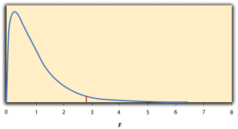
Again, the reason that F is useful is that we know how it is distributed when the null hypothesis is true. As shown in Figure 13.2, this distribution is unimodal and positively skewed with values that cluster around 1. The precise shape of the distribution depends on both the number of groups and the sample size, and there are degrees of freedom values associated with each of these. The between-groups degrees of freedom is the number of groups minus one: dfB = (G − 1). The within-groups degrees of freedom is the total sample size minus the number of groups: dfW = N − G. Again, knowing the distribution of F when the null hypothesis is true allows us to find the p value.
The online tools in Chapter 12 and statistical software such as Excel and SPSS will compute F and find the p value. If p is equal to or less than .05, then we reject the null hypothesis and conclude that there are differences among the group means in the population. If p is greater than .05, then we retain the null hypothesis and conclude that there is not enough evidence to say that there are differences. In the unlikely event that we would compute F by hand, we can use a table of critical values like Table 13.3 “Table of Critical Values of ” to make the decision. The idea is that any F ratio greater than the critical value has a p value of less than .05. Thus if the F ratio we compute is beyond the critical value, then we reject the null hypothesis. If the F ratio we compute is less than the critical value, then we retain the null hypothesis.
| dfB | |||
| dfW | 2 | 3 | 4 |
| 8 | 4.459 | 4.066 | 3.838 |
| 9 | 4.256 | 3.863 | 3.633 |
| 10 | 4.103 | 3.708 | 3.478 |
| 11 | 3.982 | 3.587 | 3.357 |
| 12 | 3.885 | 3.490 | 3.259 |
| 13 | 3.806 | 3.411 | 3.179 |
| 14 | 3.739 | 3.344 | 3.112 |
| 15 | 3.682 | 3.287 | 3.056 |
| 16 | 3.634 | 3.239 | 3.007 |
| 17 | 3.592 | 3.197 | 2.965 |
| 18 | 3.555 | 3.160 | 2.928 |
| 19 | 3.522 | 3.127 | 2.895 |
| 20 | 3.493 | 3.098 | 2.866 |
| 21 | 3.467 | 3.072 | 2.840 |
| 22 | 3.443 | 3.049 | 2.817 |
| 23 | 3.422 | 3.028 | 2.796 |
| 24 | 3.403 | 3.009 | 2.776 |
| 25 | 3.385 | 2.991 | 2.759 |
| 30 | 3.316 | 2.922 | 2.690 |
| 35 | 3.267 | 2.874 | 2.641 |
| 40 | 3.232 | 2.839 | 2.606 |
| 45 | 3.204 | 2.812 | 2.579 |
| 50 | 3.183 | 2.790 | 2.557 |
| 55 | 3.165 | 2.773 | 2.540 |
| 60 | 3.150 | 2.758 | 2.525 |
| 65 | 3.138 | 2.746 | 2.513 |
| 70 | 3.128 | 2.736 | 2.503 |
| 75 | 3.119 | 2.727 | 2.494 |
| 80 | 3.111 | 2.719 | 2.486 |
| 85 | 3.104 | 2.712 | 2.479 |
| 90 | 3.098 | 2.706 | 2.473 |
| 95 | 3.092 | 2.700 | 2.467 |
| 100 | 3.087 | 2.696 | 2.463 |
Example One-Way ANOVA
Imagine that the health psychologist wants to compare the calorie estimates of psychology majors, nutrition majors, and professional dieticians. He collects the following data:
Psych majors: 200, 180, 220, 160, 150, 200, 190, 200
Nutrition majors: 190, 220, 200, 230, 160, 150, 200, 210, 195
Dieticians: 220, 250, 240, 275, 250, 230, 200, 240
The means are 187.50 (SD = 23.14), 195.00 (SD = 27.77), and 238.13 (SD = 22.35), respectively. So it appears that dieticians made substantially more accurate estimates on average. The researcher would almost certainly enter these data into a program such as Excel or SPSS, which would compute F for him or her and find the p value. Table 13.4 shows the output of the one-way ANOVA function in Excel for these data. This table is referred to as an ANOVA table. It shows that MSB is 5,971.88, MSW is 602.23, and their ratio, F, is 9.92. The p value is .0009. Because this value is below .05, the researcher would reject the null hypothesis and conclude that the mean calorie estimates for the three groups are not the same in the population. Notice that the ANOVA table also includes the “sum of squares” (SS) for between groups and for within groups. These values are computed on the way to finding MSB and MSW but are not typically reported by the researcher. Finally, if the researcher were to compute the F ratio by hand, he could look at Table 13.3 and see that the critical value of F with 2 and 21 degrees of freedom is 3.467 (the same value in Table 13.4 under Fcrit). The fact that his F score was more extreme than this critical value would tell him that his p value is less than .05 and that he should reject the null hypothesis.
| ANOVA | ||||||
| Source of variation | SS | df | MS | F | p-value | Fcrit |
| Between groups | 11,943.75 | 2 | 5,971.875 | 9.916234 | 0.000928 | 3.4668 |
| Within groups | 12,646.88 | 21 | 602.2321 | |||
| Total | 24,590.63 | 23 | ||||
ANOVA Elaborations
Post Hoc Comparisons
When we reject the null hypothesis in a one-way ANOVA, we conclude that the group means are not all the same in the population. But this can indicate different things. With three groups, it can indicate that all three means are significantly different from each other. Or it can indicate that one of the means is significantly different from the other two, but the other two are not significantly different from each other. It could be, for example, that the mean calorie estimates of psychology majors, nutrition majors, and dieticians are all significantly different from each other. Or it could be that the mean for dieticians is significantly different from the means for psychology and nutrition majors, but the means for psychology and nutrition majors are not significantly different from each other. For this reason, statistically significant one-way ANOVA results are typically followed up with a series of post hoc comparisons of selected pairs of group means to determine which are different from which others.
One approach to post hoc comparisons would be to conduct a series of independent-samples t-tests comparing each group mean to each of the other group means. But there is a problem with this approach. In general, if we conduct a t-test when the null hypothesis is true, we have a 5% chance of mistakenly rejecting the null hypothesis (see Section 13.3 “Additional Considerations” for more on such Type I errors). If we conduct several t-tests when the null hypothesis is true, the chance of mistakenly rejecting at least one null hypothesis increases with each test we conduct. Thus researchers do not usually make post hoc comparisons using standard t-tests because there is too great a chance that they will mistakenly reject at least one null hypothesis. Instead, they use one of several modified t-test procedures—among them the Bonferonni procedure, Fisher’s least significant difference (LSD) test, and Tukey’s honestly significant difference (HSD) test. The details of these approaches are beyond the scope of this book, but it is important to understand their purpose. It is to keep the risk of mistakenly rejecting a true null hypothesis to an acceptable level (close to 5%).
Repeated-Measures ANOVA
Recall that the one-way ANOVA is appropriate for between-subjects designs in which the means being compared come from separate groups of participants. It is not appropriate for within-subjects designs in which the means being compared come from the same participants tested under different conditions or at different times. This requires a slightly different approach, called the repeated-measures ANOVA. The basics of the repeated-measures ANOVA are the same as for the one-way ANOVA. The main difference is that measuring the dependent variable multiple times for each participant allows for a more refined measure of MSW. Imagine, for example, that the dependent variable in a study is a measure of reaction time. Some participants will be faster or slower than others because of stable individual differences in their nervous systems, muscles, and other factors. In a between-subjects design, these stable individual differences would simply add to the variability within the groups and increase the value of MSW (which would, in turn, decrease the value of F). In a within-subjects design, however, these stable individual differences can be measured and subtracted from the value of MSW. This lower value of MSW means a higher value of F and a more sensitive test.
Factorial ANOVA
When more than one independent variable is included in a factorial design, the appropriate approach is the factorial ANOVA. Again, the basics of the factorial ANOVA are the same as for the one-way and repeated-measures ANOVAs. The main difference is that it produces an F ratio and p value for each main effect and for each interaction. Returning to our calorie estimation example, imagine that the health psychologist tests the effect of participant major (psychology vs. nutrition) and food type (cookie vs. hamburger) in a factorial design. A factorial ANOVA would produce separate F ratios and p values for the main effect of major, the main effect of food type, and the interaction between major and food. Appropriate modifications must be made depending on whether the design is between-subjects, within-subjects, or mixed.
Testing Correlation Coefficients
For relationships between quantitative variables, where Pearson’s r (the correlation coefficient) is used to describe the strength of those relationships, the appropriate null hypothesis test is a test of the correlation coefficient. The basic logic is exactly the same as for other null hypothesis tests. In this case, the null hypothesis is that there is no relationship in the population. We can use the Greek lowercase rho (ρ) to represent the relevant parameter: ρ = 0. The alternative hypothesis is that there is a relationship in the population: ρ ≠ 0. As with the t- test, this test can be two-tailed if the researcher has no expectation about the direction of the relationship or one-tailed if the researcher expects the relationship to go in a particular direction.
It is possible to use the correlation coefficient for the sample to compute a t score with N − 2 degrees of freedom and then to proceed as for a t-test. However, because of the way it is computed, the correlation coefficient can also be treated as its own test statistic. The online statistical tools and statistical software such as Excel and SPSS generally compute the correlation coefficient and provide the p value associated with that value. As always, if the p value is equal to or less than .05, we reject the null hypothesis and conclude that there is a relationship between the variables in the population. If the p value is greater than .05, we retain the null hypothesis and conclude that there is not enough evidence to say there is a relationship in the population. If we compute the correlation coefficient by hand, we can use a table like Table 13.5, which shows the critical values of r for various samples sizes when α is .05. A sample value of the correlation coefficient that is more extreme than the critical value is statistically significant.
| Critical value of r | ||
| N | One-tailed | Two-tailed |
| 5 | .805 | .878 |
| 10 | .549 | .632 |
| 15 | .441 | .514 |
| 20 | .378 | .444 |
| 25 | .337 | .396 |
| 30 | .306 | .361 |
| 35 | .283 | .334 |
| 40 | .264 | .312 |
| 45 | .248 | .294 |
| 50 | .235 | .279 |
| 55 | .224 | .266 |
| 60 | .214 | .254 |
| 65 | .206 | .244 |
| 70 | .198 | .235 |
| 75 | .191 | .227 |
| 80 | .185 | .220 |
| 85 | .180 | .213 |
| 90 | .174 | .207 |
| 95 | .170 | .202 |
| 100 | .165 | .197 |
Example Test of a Correlation Coefficient
Imagine that the health psychologist is interested in the correlation between people’s calorie estimates and their weight. She has no expectation about the direction of the relationship, so she decides to conduct a two-tailed test. She computes the correlation coefficient for a sample of 22 university students and finds that Pearson’s r is −.21. The statistical software she uses tells her that the p value is .348. It is greater than .05, so she retains the null hypothesis and concludes that there is no relationship between people’s calorie estimates and their weight. If she were to compute the correlation coefficient by hand, she could look at Table 13.5 and see that the critical value for 22 − 2 = 20 degrees of freedom is .444. The fact that the correlation coefficient for her sample is less extreme than this critical value tells her that the p value is greater than .05 and that she should retain the null hypothesis.
Learning Objectives
- Explain the difference between between-subjects and within-subjects experiments, list some of the pros and cons of each approach, and decide which approach to use to answer a particular research question.
- Define random assignment, distinguish it from random sampling, explain its purpose in experimental research, and use some simple strategies to implement it
- Define several types of carryover effect, give examples of each, and explain how counterbalancing helps to deal with them.
In this section, we look at some different ways to design an experiment. The primary distinction we will make is between approaches in which each participant experiences one level of the independent variable and approaches in which each participant experiences all levels of the independent variable. The former are called between-subjects experiments and the latter are called within-subjects experiments.
Between-Subjects Experiments
In a between-subjects experiment, each participant is tested in only one condition. For example, a researcher with a sample of 100 university students might assign half of them to write about a traumatic event and the other half write about a neutral event. Or a researcher with a sample of 60 people with severe agoraphobia (fear of open spaces) might assign 20 of them to receive each of three different treatments for that disorder. It is essential in a between-subjects experiment that the researcher assigns participants to conditions so that the different groups are, on average, highly similar to each other. Those in a trauma condition and a neutral condition, for example, should include a similar proportion of men and women, and they should have similar average IQs, similar average levels of motivation, similar average numbers of health problems, and so on. This matching is a matter of controlling these extraneous participant variables across conditions so that they do not become confounding variables.
Random Assignment
The primary way that researchers accomplish this kind of control of extraneous variables across conditions is called random assignment, which means using a random process to decide which participants are tested in which conditions. Do not confuse random assignment with random sampling. Random sampling is a method for selecting a sample from a population, and it is rarely used in psychological research. Random assignment is a method for assigning participants in a sample to the different conditions, and it is an important element of all experimental research in psychology and other fields too.
In its strictest sense, random assignment should meet two criteria. One is that each participant has an equal chance of being assigned to each condition (e.g., a 50% chance of being assigned to each of two conditions). The second is that each participant is assigned to a condition independently of other participants. Thus one way to assign participants to two conditions would be to flip a coin for each one. If the coin lands heads, the participant is assigned to Condition A, and if it lands tails, the participant is assigned to Condition B. For three conditions, one could use a computer to generate a random integer from 1 to 3 for each participant. If the integer is 1, the participant is assigned to Condition A; if it is 2, the participant is assigned to Condition B; and if it is 3, the participant is assigned to Condition C. In practice, a full sequence of conditions—one for each participant expected to be in the experiment—is usually created ahead of time, and each new participant is assigned to the next condition in the sequence as they are tested. When the procedure is computerized, the computer program often handles the random assignment.
One problem with coin flipping and other strict procedures for random assignment is that they are likely to result in unequal sample sizes in the different conditions. Unequal sample sizes are generally not a serious problem, and you should never throw away data you have already collected to achieve equal sample sizes. However, for a fixed number of participants, it is statistically most efficient to divide them into equal-sized groups. It is standard practice, therefore, to use a kind of modified random assignment that keeps the number of participants in each group as similar as possible. One approach is block randomization. In block randomization, all the conditions occur once in the sequence before any of them is repeated. Then they all occur again before any of them is repeated again. Within each of these “blocks,” the conditions occur in a random order. Again, the sequence of conditions is usually generated before any participants are tested, and each new participant is assigned to the next condition in the sequence. Table 5.2 shows such a sequence for assigning nine participants to three conditions. The Research Randomizer website (http://www.randomizer.org) will generate block randomization sequences for any number of participants and conditions. Again, when the procedure is computerized, the computer program often handles the block randomization.
| Participant | Condition |
| 1 | A |
| 2 | C |
| 3 | B |
| 4 | B |
| 5 | C |
| 6 | A |
| 7 | C |
| 8 | B |
| 9 | A |
Random assignment is not guaranteed to control all extraneous variables across conditions. The process is random, so it is always possible that just by chance, the participants in one condition might turn out to be substantially older, less tired, more motivated, or less depressed on average than the participants in another condition. However, there are some reasons that this possibility is not a major concern. One is that random assignment works better than one might expect, especially for large samples. Another is that the inferential statistics that researchers use to decide whether a difference between groups reflects a difference in the population takes the “fallibility” of random assignment into account. Yet another reason is that even if random assignment does result in a confounding variable and therefore produces misleading results, this confound is likely to be detected when the experiment is replicated. The upshot is that random assignment to conditions—although not infallible in terms of controlling extraneous variables—is always considered a strength of a research design.
Matched Groups
An alternative to simple random assignment of participants to conditions is the use of a matched-groups design. Using this design, participants in the various conditions are matched on the dependent variable or on some extraneous variable(s) prior the manipulation of the independent variable. This guarantees that these variables will not be confounded across the experimental conditions. For instance, if we want to determine whether expressive writing affects people's health then we could start by measuring various health-related variables in our prospective research participants. We could then use that information to rank-order participants according to how healthy or unhealthy they are. Next, the two healthiest participants would be randomly assigned to complete different conditions (one would be randomly assigned to the traumatic experiences writing condition and the other to the neutral writing condition). The next two healthiest participants would then be randomly assigned to complete different conditions, and so on until the two least healthy participants. This method would ensure that participants in the traumatic experiences writing condition are matched to participants in the neutral writing condition with respect to health at the beginning of the study. If at the end of the experiment, a difference in health was detected across the two conditions, then we would know that it is due to the writing manipulation and not to pre-existing differences in health.
Within-Subjects Experiments
In a within-subjects experiment, each participant is tested under all conditions. Consider an experiment on the effect of a defendant’s physical attractiveness on judgments of his guilt. Again, in a between-subjects experiment, one group of participants would be shown an attractive defendant and asked to judge his guilt, and another group of participants would be shown an unattractive defendant and asked to judge his guilt. In a within-subjects experiment, however, the same group of participants would judge the guilt of both an attractive and an unattractive defendant.
The primary advantage of this approach is that it provides maximum control of extraneous participant variables. Participants in all conditions have the same mean IQ, same socioeconomic status, same number of siblings, and so on—because they are the very same people. Within-subjects experiments also make it possible to use statistical procedures that remove the effect of these extraneous participant variables on the dependent variable and therefore make the data less “noisy” and the effect of the independent variable easier to detect. We will look more closely at this idea later in the book. However, not all experiments can use a within-subjects design nor would it be desirable to do so.
Carryover Effects and Counterbalancing
The primary disadvantage of within-subjects designs is that they can result in order effects. An order effect occurs when participants' responses in the various conditions are affected by the order of conditions to which they were exposed. One type of order effect is a carryover effect. A carryover effect is an effect of being tested in one condition on participants’ behavior in later conditions. One type of carryover effect is a practice effect, where participants perform a task better in later conditions because they have had a chance to practice it. Another type is a fatigue effect, where participants perform a task worse in later conditions because they become tired or bored. Being tested in one condition can also change how participants perceive stimuli or interpret their task in later conditions. This type of effect is called a context effect (or contrast effect). For example, an average-looking defendant might be judged more harshly when participants have just judged an attractive defendant than when they have just judged an unattractive defendant. Within-subjects experiments also make it easier for participants to guess the hypothesis. For example, a participant who is asked to judge the guilt of an attractive defendant and then is asked to judge the guilt of an unattractive defendant is likely to guess that the hypothesis is that defendant attractiveness affects judgments of guilt. This knowledge could lead the participant to judge the unattractive defendant more harshly because he thinks this is what he is expected to do. Or it could make participants judge the two defendants similarly in an effort to be “fair.”
Carryover effects can be interesting in their own right. (Does the attractiveness of one person depend on the attractiveness of other people that we have seen recently?) But when they are not the focus of the research, carryover effects can be problematic. Imagine, for example, that participants judge the guilt of an attractive defendant and then judge the guilt of an unattractive defendant. If they judge the unattractive defendant more harshly, this might be because of his unattractiveness. But it could be instead that they judge him more harshly because they are becoming bored or tired. In other words, the order of the conditions is a confounding variable. The attractive condition is always the first condition and the unattractive condition the second. Thus any difference between the conditions in terms of the dependent variable could be caused by the order of the conditions and not the independent variable itself.
There is a solution to the problem of order effects, however, that can be used in many situations. It is counterbalancing, which means testing different participants in different orders. The best method of counterbalancing is complete counterbalancing in which an equal number of participants complete each possible order of conditions. For example, half of the participants would be tested in the attractive defendant condition followed by the unattractive defendant condition, and others half would be tested in the unattractive condition followed by the attractive condition. With three conditions, there would be six different orders (ABC, ACB, BAC, BCA, CAB, and CBA), so some participants would be tested in each of the six orders. With four conditions, there would be 24 different orders; with five conditions there would be 120 possible orders. With counterbalancing, participants are assigned to orders randomly, using the techniques we have already discussed. Thus, random assignment plays an important role in within-subjects designs just as in between-subjects designs. Here, instead of randomly assigning to conditions, they are randomly assigned to different orders of conditions. In fact, it can safely be said that if a study does not involve random assignment in one form or another, it is not an experiment.
A more efficient way of counterbalancing is through a Latin square design which randomizes through having equal rows and columns. For example, if you have four treatments, you must have four versions. Like a Sudoku puzzle, no treatment can repeat in a row or column. For four versions of four treatments, the Latin square design would look like:
| A | B | C | D |
| B | C | D | A |
| C | D | A | B |
| D | A | B | C |
You can see in the diagram above that the square has been constructed to ensure that each condition appears at each ordinal position (A appears first once, second once, third once, and fourth once) and each condition precedes and follows each other condition one time. A Latin square for an experiment with 6 conditions would by 6 x 6 in dimension, one for an experiment with 8 conditions would be 8 x 8 in dimension, and so on. So while complete counterbalancing of 6 conditions would require 720 orders, a Latin square would only require 6 orders.
Finally, when the number of conditions is large experiments can use random counterbalancing in which the order of the conditions is randomly determined for each participant. Using this technique every possible order of conditions is determined and then one of these orders is randomly selected for each participant. This is not as powerful a technique as complete counterbalancing or partial counterbalancing using a Latin squares design. Use of random counterbalancing will result in more random error, but if order effects are likely to be small and the number of conditions is large, this is an option available to researchers.
There are two ways to think about what counterbalancing accomplishes. One is that it controls the order of conditions so that it is no longer a confounding variable. Instead of the attractive condition always being first and the unattractive condition always being second, the attractive condition comes first for some participants and second for others. Likewise, the unattractive condition comes first for some participants and second for others. Thus any overall difference in the dependent variable between the two conditions cannot have been caused by the order of conditions. A second way to think about what counterbalancing accomplishes is that if there are carryover effects, it makes it possible to detect them. One can analyze the data separately for each order to see whether it had an effect.
When 9 Is “Larger” Than 221
Researcher Michael Birnbaum has argued that the lack of context provided by between-subjects designs is often a bigger problem than the context effects created by within-subjects designs. To demonstrate this problem, he asked participants to rate two numbers on how large they were on a scale of 1-to-10 where 1 was “very very small” and 10 was “very very large”. One group of participants were asked to rate the number 9 and another group was asked to rate the number 221 (Birnbaum, 1999)[1]. Participants in this between-subjects design gave the number 9 a mean rating of 5.13 and the number 221 a mean rating of 3.10. In other words, they rated 9 as larger than 221! According to Birnbaum, this difference is because participants spontaneously compared 9 with other one-digit numbers (in which case it is relatively large) and compared 221 with other three-digit numbers (in which case it is relatively small).
Simultaneous Within-Subjects Designs
So far, we have discussed an approach to within-subjects designs in which participants are tested in one condition at a time. There is another approach, however, that is often used when participants make multiple responses in each condition. Imagine, for example, that participants judge the guilt of 10 attractive defendants and 10 unattractive defendants. Instead of having people make judgments about all 10 defendants of one type followed by all 10 defendants of the other type, the researcher could present all 20 defendants in a sequence that mixed the two types. The researcher could then compute each participant’s mean rating for each type of defendant. Or imagine an experiment designed to see whether people with social anxiety disorder remember negative adjectives (e.g., “stupid,” “incompetent”) better than positive ones (e.g., “happy,” “productive”). The researcher could have participants study a single list that includes both kinds of words and then have them try to recall as many words as possible. The researcher could then count the number of each type of word that was recalled.
Between-Subjects or Within-Subjects?
Almost every experiment can be conducted using either a between-subjects design or a within-subjects design. This possibility means that researchers must choose between the two approaches based on their relative merits for the particular situation.
Between-subjects experiments have the advantage of being conceptually simpler and requiring less testing time per participant. They also avoid carryover effects without the need for counterbalancing. Within-subjects experiments have the advantage of controlling extraneous participant variables, which generally reduces noise in the data and makes it easier to detect any effect of the independent variable upon the dependent variable. Within-subjects experiments also require fewer participants than between-subjects experiments to detect an effect of the same size.
A good rule of thumb, then, is that if it is possible to conduct a within-subjects experiment (with proper counterbalancing) in the time that is available per participant—and you have no serious concerns about carryover effects—this design is probably the best option. If a within-subjects design would be difficult or impossible to carry out, then you should consider a between-subjects design instead. For example, if you were testing participants in a doctor’s waiting room or shoppers in line at a grocery store, you might not have enough time to test each participant in all conditions and therefore would opt for a between-subjects design. Or imagine you were trying to reduce people’s level of prejudice by having them interact with someone of another race. A within-subjects design with counterbalancing would require testing some participants in the treatment condition first and then in a control condition. But if the treatment works and reduces people’s level of prejudice, then they would no longer be suitable for testing in the control condition. This difficulty is true for many designs that involve a treatment meant to produce long-term change in participants’ behavior (e.g., studies testing the effectiveness of psychotherapy). Clearly, a between-subjects design would be necessary here.
Remember also that using one type of design does not preclude using the other type in a different study. There is no reason that a researcher could not use both a between-subjects design and a within-subjects design to answer the same research question. In fact, professional researchers often take exactly this type of mixed methods approach.
Involves measuring several variables (X1, X2, X3,…Xi), and using them to predict some outcome variable (Y).
The extent to which people’s scores on a measure are correlated with other variables (known as criteria) that one would expect them to be correlated with.
A quantitative and qualitative method with two important characteristics; variables are measured using self-reports and considerable attention is paid to the issue of sampling.
Learning Objectives
- Explain what an experiment is and recognize examples of studies that are experiments and studies that are not experiments.
- Distinguish between the manipulation of the independent variable and control of extraneous variables and explain the importance of each.
- Recognize examples of confounding variables and explain how they affect the internal validity of a study.
- Define what a control condition is, explain its purpose in research on treatment effectiveness, and describe some alternative types of control conditions.
What Is an Experiment?
As we saw earlier in the book, an experiment is a type of study designed specifically to answer the question of whether there is a causal relationship between two variables. In other words, whether changes in one variable (referred to as an independent variable) cause a change in another variable (referred to as a dependent variable). Experiments have two fundamental features. The first is that the researchers manipulate, or systematically vary, the level of the independent variable. The different levels of the independent variable are called conditions. For example, in Darley and Latané’s experiment, the independent variable was the number of witnesses that participants believed to be present. The researchers manipulated this independent variable by telling participants that there were either one, two, or five other students involved in the discussion, thereby creating three conditions. For a new researcher, it is easy to confuse these terms by believing there are three independent variables in this situation: one, two, or five students involved in the discussion, but there is actually only one independent variable (number of witnesses) with three different levels or conditions (one, two or five students). The second fundamental feature of an experiment is that the researcher exerts control over, or minimizes the variability in, variables other than the independent and dependent variable. These other variables are called extraneous variables. Darley and Latané tested all their participants in the same room, exposed them to the same emergency situation, and so on. They also randomly assigned their participants to conditions so that the three groups would be similar to each other to begin with. Notice that although the words manipulation and control have similar meanings in everyday language, researchers make a clear distinction between them. They manipulate the independent variable by systematically changing its levels and control other variables by holding them constant.
Manipulation of the Independent Variable
Again, to manipulate an independent variable means to change its level systematically so that different groups of participants are exposed to different levels of that variable, or the same group of participants is exposed to different levels at different times. For example, to see whether expressive writing affects people’s health, a researcher might instruct some participants to write about traumatic experiences and others to write about neutral experiences. The different levels of the independent variable are referred to as conditions, and researchers often give the conditions short descriptive names to make it easy to talk and write about them. In this case, the conditions might be called the “traumatic condition” and the “neutral condition.”
Notice that the manipulation of an independent variable must involve the active intervention of the researcher. Comparing groups of people who differ on the independent variable before the study begins is not the same as manipulating that variable. For example, a researcher who compares the health of people who already keep a journal with the health of people who do not keep a journal has not manipulated this variable and therefore has not conducted an experiment. This distinction is important because groups that already differ in one way at the beginning of a study are likely to differ in other ways too. For example, people who choose to keep journals might also be more conscientious, more introverted, or less stressed than people who do not. Therefore, any observed difference between the two groups in terms of their health might have been caused by whether or not they keep a journal, or it might have been caused by any of the other differences between people who do and do not keep journals. Thus the active manipulation of the independent variable is crucial for eliminating potential alternative explanations for the results.
Of course, there are many situations in which the independent variable cannot be manipulated for practical or ethical reasons and therefore an experiment is not possible. For example, whether or not people have a significant early illness experience cannot be manipulated, making it impossible to conduct an experiment on the effect of early illness experiences on the development of hypochondriasis. This caveat does not mean it is impossible to study the relationship between early illness experiences and hypochondriasis—only that it must be done using nonexperimental approaches. We will discuss this type of methodology in detail later in the book.
Independent variables can be manipulated to create two conditions and experiments involving a single independent variable with two conditions are often referred to as a single factor two-level design. However, sometimes greater insights can be gained by adding more conditions to an experiment. When an experiment has one independent variable that is manipulated to produce more than two conditions it is referred to as a single factor multi level design. So rather than comparing a condition in which there was one witness to a condition in which there were five witnesses (which would represent a single-factor two-level design), Darley and Latané’s experiment used a single factor multi-level design, by manipulating the independent variable to produce three conditions (a one witness, a two witnesses, and a five witnesses condition).
Control of Extraneous Variables
As we have seen previously in the chapter, an extraneous variable is anything that varies in the context of a study other than the independent and dependent variables. In an experiment on the effect of expressive writing on health, for example, extraneous variables would include participant variables (individual differences) such as their writing ability, their diet, and their gender. They would also include situational or task variables such as the time of day when participants write, whether they write by hand or on a computer, and the weather. Extraneous variables pose a problem because many of them are likely to have some effect on the dependent variable. For example, participants’ health will be affected by many things other than whether or not they engage in expressive writing. This influencing factor can make it difficult to separate the effect of the independent variable from the effects of the extraneous variables, which is why it is important to control extraneous variables by holding them constant.
Extraneous Variables as “Noise”
Extraneous variables make it difficult to detect the effect of the independent variable in two ways. One is by adding variability or “noise” to the data. Imagine a simple experiment on the effect of mood (happy vs. sad) on the number of happy childhood events people are able to recall. Participants are put into a negative or positive mood (by showing them a happy or sad video clip) and then asked to recall as many happy childhood events as they can. The two leftmost columns of Table 5.1 show what the data might look like if there were no extraneous variables and the number of happy childhood events participants recalled was affected only by their moods. Every participant in the happy mood condition recalled exactly four happy childhood events, and every participant in the sad mood condition recalled exactly three. The effect of mood here is quite obvious. In reality, however, the data would probably look more like those in the two rightmost columns of Table 5.1. Even in the happy mood condition, some participants would recall fewer happy memories because they have fewer to draw on, use less effective recall strategies, or are less motivated. And even in the sad mood condition, some participants would recall more happy childhood memories because they have more happy memories to draw on, they use more effective recall strategies, or they are more motivated. Although the mean difference between the two groups is the same as in the idealized data, this difference is much less obvious in the context of the greater variability in the data. Thus one reason researchers try to control extraneous variables is so their data look more like the idealized data in Table 5.1, which makes the effect of the independent variable easier to detect (although real data never look quite that good).
| Idealized “noiseless” data | Realistic “noisy” data | ||
| Happy mood | Sad mood | Happy mood | Sad mood |
| 4 | 3 | 3 | 1 |
| 4 | 3 | 6 | 3 |
| 4 | 3 | 2 | 4 |
| 4 | 3 | 4 | 0 |
| 4 | 3 | 5 | 5 |
| 4 | 3 | 2 | 7 |
| 4 | 3 | 3 | 2 |
| 4 | 3 | 1 | 5 |
| 4 | 3 | 6 | 1 |
| 4 | 3 | 8 | 2 |
| M = 4 | M = 3 | M = 4 | M = 3 |
One way to control extraneous variables is to hold them constant. This technique can mean holding situation or task variables constant by testing all participants in the same location, giving them identical instructions, treating them in the same way, and so on. It can also mean holding participant variables constant. For example, many studies of language limit participants to right-handed people, who generally have their language areas isolated in their left cerebral hemispheres[2]. Left-handed people are more likely to have their language areas isolated in their right cerebral hemispheres or distributed across both hemispheres, which can change the way they process language and thereby add noise to the data.
In principle, researchers can control extraneous variables by limiting participants to one very specific category of person, such as 20-year-old, heterosexual, female, right-handed psychology majors. The obvious downside to this approach is that it would lower the external validity of the study—in particular, the extent to which the results can be generalized beyond the people actually studied. For example, it might be unclear whether results obtained with a sample of younger lesbian women would apply to older gay men. In many situations, the advantages of a diverse sample (increased external validity) outweigh the reduction in noise achieved by a homogeneous one.
Extraneous Variables as Confounding Variables
The second way that extraneous variables can make it difficult to detect the effect of the independent variable is by becoming confounding variables. A confounding variable is an extraneous variable that differs on average across levels of the independent variable (i.e., it is an extraneous variable that varies systematically with the independent variable). For example, in almost all experiments, participants’ intelligence quotients (IQs) will be an extraneous variable. But as long as there are participants with lower and higher IQs in each condition so that the average IQ is roughly equal across the conditions, then this variation is probably acceptable (and may even be desirable). What would be bad, however, would be for participants in one condition to have substantially lower IQs on average and participants in another condition to have substantially higher IQs on average. In this case, IQ would be a confounding variable.
To confound means to confuse, and this effect is exactly why confounding variables are undesirable. Because they differ systematically across conditions—just like the independent variable—they provide an alternative explanation for any observed difference in the dependent variable. Figure 5.1 shows the results of a hypothetical study, in which participants in a positive mood condition scored higher on a memory task than participants in a negative mood condition. But if IQ is a confounding variable—with participants in the positive mood condition having higher IQs on average than participants in the negative mood condition—then it is unclear whether it was the positive moods or the higher IQs that caused participants in the first condition to score higher. One way to avoid confounding variables is by holding extraneous variables constant. For example, one could prevent IQ from becoming a confounding variable by limiting participants only to those with IQs of exactly 100. But this approach is not always desirable for reasons we have already discussed. A second and much more general approach—random assignment to conditions—will be discussed in detail shortly.

Treatment and Control Conditions
In psychological research, a treatment is any intervention meant to change people’s behavior for the better. This intervention includes psychotherapies and medical treatments for psychological disorders but also interventions designed to improve learning, promote conservation, reduce prejudice, and so on. To determine whether a treatment works, participants are randomly assigned to either a treatment condition, in which they receive the treatment, or a control condition, in which they do not receive the treatment. If participants in the treatment condition end up better off than participants in the control condition—for example, they are less depressed, learn faster, conserve more, express less prejudice—then the researcher can conclude that the treatment works. In research on the effectiveness of psychotherapies and medical treatments, this type of experiment is often called a randomized clinical trial.
There are different types of control conditions. In a no-treatment control condition, participants receive no treatment whatsoever. One problem with this approach, however, is the existence of placebo effects. A placebo is a simulated treatment that lacks any active ingredient or element that should make it effective, and a placebo effect is a positive effect of such a treatment. Many folk remedies that seem to work—such as eating chicken soup for a cold or placing soap under the bed sheets to stop nighttime leg cramps—are probably nothing more than placebos. Although placebo effects are not well understood, they are probably driven primarily by people’s expectations that they will improve. Having the expectation to improve can result in reduced stress, anxiety, and depression, which can alter perceptions and even improve immune system functioning (Price, Finniss, & Benedetti, 2008)[3].
Placebo effects are interesting in their own right (see Note "The Powerful Placebo"), but they also pose a serious problem for researchers who want to determine whether a treatment works. Figure 5.2 shows some hypothetical results in which participants in a treatment condition improved more on average than participants in a no-treatment control condition. If these conditions (the two leftmost bars in Figure 5.2) were the only conditions in this experiment, however, one could not conclude that the treatment worked. It could be instead that participants in the treatment group improved more because they expected to improve, while those in the no-treatment control condition did not.
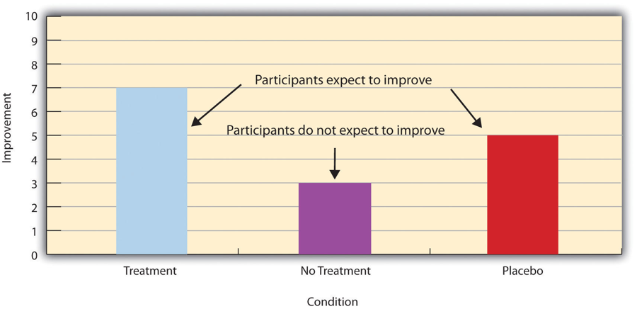
Fortunately, there are several solutions to this problem. One is to include a placebo control condition, in which participants receive a placebo that looks much like the treatment but lacks the active ingredient or element thought to be responsible for the treatment’s effectiveness. When participants in a treatment condition take a pill, for example, then those in a placebo control condition would take an identical-looking pill that lacks the active ingredient in the treatment (a “sugar pill”). In research on psychotherapy effectiveness, the placebo might involve going to a psychotherapist and talking in an unstructured way about one’s problems. The idea is that if participants in both the treatment and the placebo control groups expect to improve, then any improvement in the treatment group over and above that in the placebo control group must have been caused by the treatment and not by participants’ expectations. This difference is what is shown by a comparison of the two outer bars in Figure 5.4.
Of course, the principle of informed consent requires that participants be told that they will be assigned to either a treatment or a placebo control condition—even though they cannot be told which until the experiment ends. In many cases the participants who had been in the control condition are then offered an opportunity to have the real treatment. An alternative approach is to use a wait-list control condition, in which participants are told that they will receive the treatment but must wait until the participants in the treatment condition have already received it. This disclosure allows researchers to compare participants who have received the treatment with participants who are not currently receiving it but who still expect to improve (eventually). A final solution to the problem of placebo effects is to leave out the control condition completely and compare any new treatment with the best available alternative treatment. For example, a new treatment for simple phobia could be compared with standard exposure therapy. Because participants in both conditions receive a treatment, their expectations about improvement should be similar. This approach also makes sense because once there is an effective treatment, the interesting question about a new treatment is not simply “Does it work?” but “Does it work better than what is already available?
The Powerful Placebo
Many people are not surprised that placebos can have a positive effect on disorders that seem fundamentally psychological, including depression, anxiety, and insomnia. However, placebos can also have a positive effect on disorders that most people think of as fundamentally physiological. These include asthma, ulcers, and warts (Shapiro & Shapiro, 1999)[4]. There is even evidence that placebo surgery—also called “sham surgery”—can be as effective as actual surgery.
Medical researcher J. Bruce Moseley and his colleagues conducted a study on the effectiveness of two arthroscopic surgery procedures for osteoarthritis of the knee (Moseley et al., 2002)[5]. The control participants in this study were prepped for surgery, received a tranquilizer, and even received three small incisions in their knees. But they did not receive the actual arthroscopic surgical procedure. Note that the IRB would have carefully considered the use of deception in this case and judged that the benefits of using it outweighed the risks and that there was no other way to answer the research question (about the effectiveness of a placebo procedure) without it. The surprising result was that all participants improved in terms of both knee pain and function, and the sham surgery group improved just as much as the treatment groups. According to the researchers, “This study provides strong evidence that arthroscopic lavage with or without débridement [the surgical procedures used] is not better than and appears to be equivalent to a placebo procedure in improving knee pain and self-reported function” (p. 85).
