Introduction

Daniel FitzGreen

Quantum Analogs

Introduction

2.1 Standing Waves

Waves are everywhere, and even when they aren’t perfect solutions, they’re an easy way to learn more about a problem. If some experimentalist out there has a signal that’s changing in time, then there’s probably some theorist out there using a wave to approximate it.

Quantum mechanical states are described using wavefunctions, typically denoted as $\psi$ . Wavefunctions contain all the useful information about the quantum particle as as its position, momentum, energy, etc… Wavefunctions are determined by solving Shroedinger’s equation:

(1) $\begin{equation*} i\hbar \cfrac{\partial\psi(r,t)}{\partial t}=\cfrac{\hbar^2}{2m}\Delta\psi (r,t) + V(r)\psi (r,t).\end{equation*}$

A common example quantum system is the particle-in-a-box: A single particle trapped by a 1-D potential $V(x)$ where $V(|x|<a) = 0$ and $V(|x|>a)=\infty$ for a potential well of length $a$ . The amplitude of the wavefunction ( $\psi(x,t)$ ) describes the probability of finding the quantum particle in a given range of locations $(|\psi(x_1<x<x_2)|^2$ = some number less than one) at some time $t$ . If you haven’t seen this in an intro quantum mechanics course, you will soon. This simple example system has an analytical solution and can be used to approximate much more mathematically-complicated systems such as those found in atoms and molecules.

Since $V(x) = 0$ inside the well, Schroedingers equation has a pretty simple solution: a free particle:

(2) $\begin{equation*} \psi(x,t) = [A\sin (kx) + B\cos (kx)] * \exp [-i\omega t], \end{equation*}$

where $k$ is some integer $n$ of $\pi/L$ ’s so that the amplitude of the function is zero at the well boundaries. That solution contains function we would expect to find in some kind of wave!!!!1! What are the odds!?!? (about 1/1). The time dependence is irrelevant for now since nothing about out potential well is changing in time – we’re looking at standing waves here. You can find this derivation in literally every introductory quantum textbook. I’ll jump to the conclusion: The wavefunction for the particle in the box and its eigenvalues (energies) are:

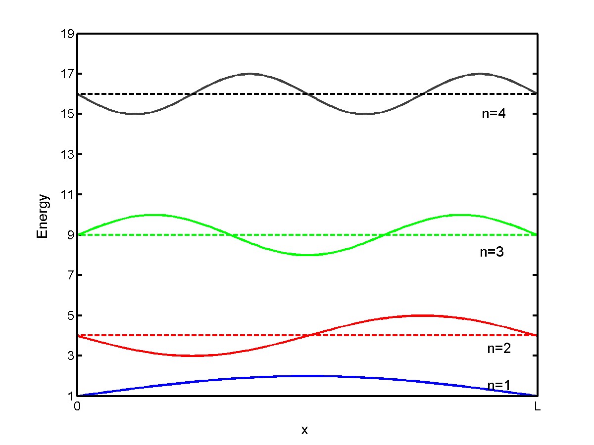
(3) $\begin{align*} \phi &= \sin (n\pi x/L); \\ E_n &= \cfrac{n^2\hbar^2\pi^2}{2mL^2},\end{align*}$

Figure 1: Example solution to the particle in a box. Note the discrete energy levels. Figure from Wikipedia.

where $n$ is the energy level of the standing wave (some examples are shown in Figure 1), $L$ is the length of the potential well, and $m$ is the mass of the particle. Figure 1 sure does look like a bunch of integer-number of wavelengths; sure does look like the standing wave you would get from vibrations on a strong, or vibrations through a fluid like water…or even air!

The analogous energy levels of a standing sound wave in a finite tube are the allowed frequencies:

(4) $\begin{equation*} f =\cfrac{nv}{2L},\end{equation*}$

where $v$ is the speed of the wave. Note the difference in the $n$ dependence. Since we know the frequencies that result in a standing wave, we know the wavelengths:

(5) $\begin{equation*} \lambda = \cfrac{2L}{n}. \end{equation*}$

And then we define the wavenumber, which will be used to characterize energy levels in solid-state physics:

(6) $\begin{equation*} k = \cfrac{2\pi}{\lambda} = n\cfrac{\pi}{L}\end{equation*}$

2.2 Dispersion Relation

The dispersion relation of a wave relates the wavelength or wavenumber of a wave to its frequency. In the above example of a particle in a box, the dispersion relation is the result of combing equations (6) and (3):

(7) $\begin{equation*} E = \cfrac{\hbar^2 k^2}{2m}.\end{equation*}$

In quantum systems, frequency and energy are often synonymous. For the standing wave in the tube, the dispersion relation is

(8) $\begin{equation*} f(k) = \cfrac{v}{2\pi}k.\end{equation*}$

Again, note the difference in $k$ dependence.

The density of states is the number of states per unit frequency that fulfill the resonant condition. In the standing wave in the tube, the dispersion relation is linear, and so the density of states is a constant. In the quantum particle in a box, the density of states increases quadratically with increasing frequency. Ask yourself how the density of states changes as a function of the tube length.

2.3 Crystal Lattice

We can build off of the very simple and boring flat potential/tube and add periodic scattering sites; like the ones you would find in a crystal lattice. When the wavelength of the incoming wave is comparable to the distance between the scattering sites, then a resonant condition is formed and incoming wave is reflected, as if by a mirror or some other perfect reflector. This type of reflection is called Bragg diffraction. The Bragg condition is

(9) $\begin{equation*} n\lambda = 2\sin\theta, \end{equation*}$

where $d$ is the distance between the scattering sites and $\theta$ is the angle of the incoming wave (In the tube, what is the value of $\theta$ ?). When the Bragg condition is met, the wave is reflected. When the Bragg condition is not met, then a gap is generated in frequency space. We call this a band gap.

It turns out that it’s mathematically inconvenient to keep describing this physics in frequency space. Instead, solid-state physicists use ‘reciprocal space’. Presuming the Bragg condition is fulfilled, a wave with wavenumber $k$ is reflected and $k \rightarrow k'$ . The difference is called the ‘reciprocal lattice vector’: $k-k'=G$ . In the 1D space of the tube $k$ changes to $-k$ , where $k$ fulfils our Bragg condition: $k=n\pi/d$ . The reciprocal vectors are then

(10) $\begin{equation*} G = n\cfrac{2\pi}{d},\end{equation*}$

where $n$ can be a positive or negative integer, or zero, and $d$ is the distance between scattering sites, which the manual denotes as $a$ . These vectors generate a ‘reciprocal lattice’, as shown in Figure 2. The unit cells of this reciprocal space are called Brillouin zones. Each zone has $2L/d$ discrete $k$ -points, but since $L$ is made up of some integer of $d$ ‘s, then one can conclude that the number of discrete $k$ -points in a Brillouin zone is twice the number of unit cells, as shown in Figure 3. Many physicists only worry about the first Brillouin zone, and call such a simplification the ‘reduced zone scheme’.

I know that the Brillouin zone stuff can be confusing at first. You can check out the TeachSpin manual or Wikipedia for supplementary info.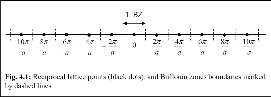

Figure 2: An illustration of reciprocal space from the TreachSpin manual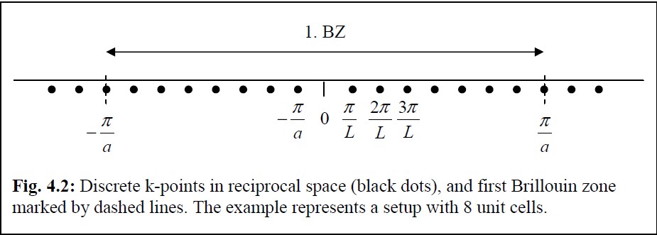

Figure 3: Discrete k-points in the first Brillouin zone.

Introduction

2.1 Standing Waves

2.2 Dispersion Relation

2.3 Crystal Lattice

License

Share This Book