PART 1: Discharging the capacitor
Part 1 is divided into two sections. The first section of Part 1 will involve determining the time constant  for the discharging RC circuit. The second section is dedicated to finding the capacitance for our capacitor through linear regression of the voltage versus time plot.
PROCEDURE
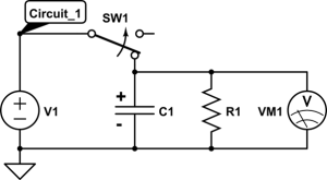
Construct Circuit_1 as shown above. Make sure the capacitor’s polarity is correctly indicated as shown in Circuit_1. The white band with minus signs on the capacitor indicates the negative side. Always connect the circuit so that the voltage across the capacitor is negative at this end and positive at the other.
The SW1 circuit element is a switch which allows you to open and close the circuit as intended. There is a PASCO circuit building block which acts like a switch.
Finding the Time Constant
This part of the procedure is dedicated to finding the time it takes for the voltage on the capacitor to reduce to half of its initial value (the time constant ).
1. Construct Circuit_1 by using the  resistor and making sure the capacitor’s polarity is correctly oriented.
 ****WARNING****
(Ask the lab coordinator or instructional assistant to check the polarity of your Capacitor in the circuit. YOU MUST, have this cleared by the lab coordinator or instructional assistant before turning on the power supply)
2. Set the power supply within Capstone to the settings:
a. Waveform = DC.
b. DC Voltage=8V (this will change later on in the procedure) and turn it on.
c. At the bottom of the page, set the frequency of measurement for the Wireless Voltage Sensor to 10Hz (this will record a value for voltage every 0.1 seconds).
3. Close the circuit with the switch (closing the circuit means it is connected) and measure the voltage across the resistor. When the capacitor (or resistor, since they are in parallel) is at the voltage of the power supply, open the circuit but continue recording. You can end the recording when the voltage begins to asymptote to zero.
a. Note: your voltage should look like a negative exponential function over time which starts at the initial voltage.
4. Double click on any point on the curve and select the “Add Coordinate” option. Here you will find the time it takes for the voltage across the resistor to drop to half of its initial value ( :
a. Select the time when the voltage begins to drop from its initial value.
b. Select the time when the voltage is half of its initial value.
c. Take the difference between the two times found in steps a and b.
Record this value in your report. For the  at an initial voltage of 8V, save this run on a separate tab in Capstone. You do not need to save the next set of runs, only this one. We will be using this set of data in the next section. If something goes wrong saving the data, you will be able to quickly re-take it later.
You can “save” your data by creating a new tab by selecting the “Add Page” option just above “Tools” on the left hand side. Then, add a new graph to this tab and plot Voltage vs. time. Your latest data Run should then be plotted on this graph. If you return to your other tab and take new data on that tab, the Run you should saved should be preserved on the new tab.
Or, you can select the entire graph area, then click the “copy” button in the very top toolbar under Edit. Then create a new tab by selecting the “Add Page” option just above “Tools” on the left. In the new tab click “paste” in the very top toolbar under Edit to paste your graph. ** Important ** Under this new tab, select the properties icon from the graph toolbar, then Data Options, then deselect both “Show New Runs” and “Show New Runs From Prior Pages”. This will allow that tab to store any of the previous runs you had without it being overwritten by the latest run.
CHECKPOINT
(Ask the TA to double check your circuit and the  value)
5. Repeat steps 1-3 with the power supply set to 6V and then with the power supply set to 4V. In the report, calculate the average and standard deviation of for that resistor’s value with the different voltage values. Use this standard deviation as the uncertainty for your value.
a. Note: make your life easier and use Excel to calculate these standard deviations for you. You can use the STDEV() function and select the values for into the functions arguments. You can also calculate the average value using the AVG() function in Excel.
6. Use resistors  and
and  and repeat steps 1-4. Calculate the capacitance C for each of these resistors by using equation (8) and your measured values. Record the value of your capacitance for each resistor in the report. Then calculate the average value for the capacitors and add it to your report.
Question 1
value seem to depend on the initial voltage? Justify your answer.
Question 2
Linear Regression with Voltage versus Time
Using Circuit_1, with  and an initial voltage of 8V, we are going to apply linear regression to a voltage versus time curve.
1. If you did not save your first curve, recreate the voltage versus time graph for  at an initial voltage of 8V at 10Hz. You can refer to the previous procedure on how to do this.
2. Take the data and prepare it for linear regression.
a. Remove every data point that is at  besides the last one. This last data point will be your initial time
  , so record its value in the report. To remove some data from your graph:
i. Select the option “Highlight range of points in active data” (this icon looks like a series of highlighted points) and cover the highlighted box over the desired data to be deleted. You can move and resize the box as needed. Then right click the highlighted box and select “Deletions  Delete Highlighted Data Points”.
b. Remove every data point that is after  . Use the average value of you previously calculated for
  .
.
3. Export the data for this graph and import it into Excel. To do this:
a. Select “File” tab within Capstone and then “Export Data”. The data file generated should automatically be in a comma separated value (CSV) format.
b. Select “Export to file” in bottom right corner. Name the file an appropriate name and save it to your local directory (folder).
c. Right click on the csv file you just saved. Then go to “open with” “Microsoft Excel”.
4. With the data imported into Excel, now we are going to create new columns for  and for
  . For the
  column:
a. Write a title for at the top of the column (don’t worry about units).
b. Write a function in the cell that takes in the adjacent Voltage value cell (probably B2 for your imported data set) and apply the natural logarithm function. You need to do this for the first two cells in the column. Excel’s built in natural logarithm function is given LN () .
i. To enter a numeric function into Excel, don’t forget to start with an equal sign, for example, type: “=LN(B2)” to calculate the natural logarithm of the B2 value.
ii. Each row entry in the column should look something like: = LN(B2), = LN(B3), …
c. Select two of the cells in the column and autofill the remaining rows by double clicking on the bottom right square. This will automatically fill in each row based on the adjacent row values in the column.
5. For the  column, write every value with respect to
  , since that is where the exponential decay started. To do this within Excel:
a. Write a title of at the top of the column with SI units of seconds.
b. Write a function in the cell that takes in the adjacent time value cell (probably A2 for your imported data set) and subtract by the constant value of .
i. Your function should look like: “ ” where is your initial time. Each entry in the column should look something like: ,
  , etc.
c. Select two of the cells in the column and autofill the remaining rows by double clicking on the bottom right square. This will automatically fill in each row based on the adjacent row values in the column.
CHECKPOINT
(Ask the TA to check your Excel file and see if you properly calculated the  and
and  columns.)
6. Create a plot of  versus time for a domain of
 ![\mathbf{t \varepsilon [t_0, t_0 + 2 \tau_{\frac{1}{2}}]}](https://ecampusontario.pressbooks.pub/app/uploads/quicklatex/quicklatex.com-b1a7c41460e552a244a16c96613d5dc5_l3.png "Rendered by QuickLaTeX.com") from the loaded data in Excel. There are multiple ways to do this, but the easiest is to:
from the loaded data in Excel. There are multiple ways to do this, but the easiest is to:
a. Click the “Insert” tab “Charts” “Insert Scatter (X,Y) or Bubble Chart” “Scatter”.
b. Right click the empty graph, select “Select Data” “Add”.
c. Left click under “Series X values:” highlight the current column. Likewise, do this for the “Series Y values:” for the Voltage column.
7. Give your plot a title and appropriate axis labels. To do this:
a. Left click anywhere on the graph, select “Chart Design” tab, then select “Add Chart Elements”.
8. Insert a trendline on the graph and display the equation &  value on the graph. To do this:
a. Right click the data series in the graph, select “Add Trendline…” “Display Equation on chart” “Display R-squared value on chart”.
9. Use the slope of the trendline you just found, along with Equation (6a), to determine the capacitance of your circuit. Add your plot to the report. Make sure your plot has properly labelled axes and titles.
***CAUTION*** Make sure you are using the natural logarithm function in Excel and that your time is properly plotted with respect to.
Equation (6a) is given as  .
.
Question 3
Question 4
.