a) Let us consider again the measurement from the digital balance we talked about in the Type B Evaluation lab.

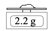
The type B evaluation gives us a minimum and maximum value of the possible reading, but ANY value between those limits is equally likely. The probability density function for this measurement might look like this:

We’ll call this a “rectangular PDF”. Assuming that the meter is rounding, label the 6 pieces of information on the plot with the bank of option above (you won’t use all the options!). Specifically, make sure you understand: 

i) what are the units on the horizontal axis? the vertical axis?

ii) what are the values at the centre and edge of the non-zero part of the function?

iii) what is the value of the probability density when it is non-zero?

b) What about a measurement on an analogue scale, like a ruler (here labelled in cm)?

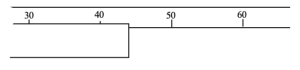
In this case, you have a most likely value, say 44 cm, and as you move further to left or right, the likelihood falls, eventually dropping to zero at 43 cm and 45 cm. An appropriate PDF for this measurement might be…

We’ll call this a “triangular PDF”. Again, label the 6 pieces of information on the plot with the bank of option above (you won’t use all the options!). Specifically, make sure you understand:

i) What are the units on the horizontal axis? the vertical axis?

ii) What are the values at the centre and edge of the non-zero part of the function?

iii) What is the value of the probability density at the peak?

c) If you have any background in statistics, you’ll know that the most common type of PDF to associate with a set of data with intrinsic randomness is the Gaussian function.

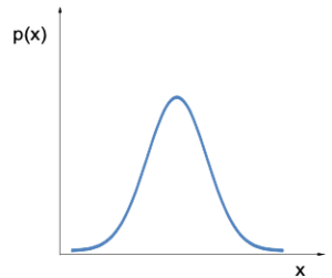
Mathematically, the Gaussian function takes the form

where p₀, x₀, and σ are constants.

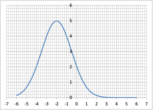
Before discussing the Gaussian PDF any further, it would be best if you familiarized yourself with the function by playing with it in Excel. Download the Gaussian PDF spreadsheet. The function p(x) is already set up and plotted for you. At the moment, the constants in the Gaussian function are set to

p₀ = 1 , x₀ = 0, and σ = 1

(You will see them at the top of the spreadsheet in cells D2, E2, F2.) Try changing the magnitudes of the variables in these cells, maybe one at a time to start with, to see how they affect the plotted function. (Just type over any of the current values and hit enter). Now go back to the function and make sure these changes are consistent with your observations.

i) If you let (x-x₀) = σ in Eq. 1 above, what is the value of p? Verify thatyour Excel plot shows the correct value of p at σ.

ii) When you are sure that you understand how the variables p₀, x₀, and σ control the function, write an equation that describes the Gaussian plotted in the image below.

iii) If the Gaussian function is to be a proper PDF, the area under the curve must be one.

Return to the original set of variables, i.e p₀ = 1 , x₀ = 0, and σ = 1. If you were to approximate the function by a triangle, what is its area? How then would you normalize the area to one?

The proper normalization constant, obtained from integration, is

How does this compare to your estimate?