Deriving the dipole potential approximation

Physics 1AA3 Team

Deriving the dipole potential approximation

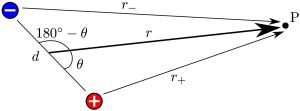
Figure 5: Same as Figure 2, this is the geometry of the dipole that will be referenced here when deriving the equation for the approximate potential (Equation 3).

Here, we go through a derivation of the approximate dipole electric potential that is studied in this experiment. This exercise isn’t required reading for this lab. It is just supplementary material for those curious about where this mathematical approximation comes from.

As stated in the introduction section, we can write down a complete and perfectly accurate expression for the electric potential around a dipole as just the sum of the individual potentials created from the two point charges:

(4) $\begin{equation*} V = V_+ (r_+) + V_- (r_-) , \end{equation*}$

(5) $\begin{equation*} = \frac{k q}{r_+} - \frac{k q}{r_-}. \end{equation*}$

It would be more useful, though, if we could write an expression for this potential that only depended on one distance from the dipole, and not two separately: $r_+$ and $r_-$ . We may also imagine that, if we were far enough away from the dipole so that we could barely measure or see the distance that separates the two charges, it is likely that we could mathematically approximate the two charges as one object to high accuracy. This is the motivation for the derivation of our approximation. Let’s begin!

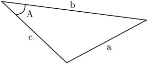
Figure 6: An example triangle for demonstrating the cosine law.

Our first task is to rewrite $r_+$ and $r_-$ r₊ in terms of (1) the separation between the charges, $d$ , (2) the distance $r$ from the centre of the dipole to the point of interest, $P$ , where we wish to approximate the potential, and (3) the angle between $r$ and $d$ , which we call $theta$ . See Figure 5 to remind yourself of the geometry. Note: we will soon make assumptions that $r >> d$ , even though visually this does not seem to be true in this schematic. The diagram is drawn for the scenario where $P$ is close to the dipole in order to make the geometry easier to see.

To accomplish this task, we can use the cosine law, true for any triangle. Figure 6 shows a general triangle, and the cosine law gives the following relation between the side lengths and angle A,

$a^2 = b^2 +c^2 - 2 bc ~\cos A.$

We can make two triangles in our dipole geometry after splitting the length $d$ in half, and then via the cosine law we have the following relations for $r_+$ and $r_-$ ,

(6) $\begin{align*} r_+^2 &= r^2 + \left(\frac{d}{2} \right)^2 - r d \cos \theta, \\ r_-^2 &= r^2 + \left(\frac{d}{2} \right)^2 - r d \cos (180 \degree -\theta), \end{align*}$

Factoring out $r^2$ from all terms on the right side of equation 6a and taking a square root of both sides, we get,

$r_+ = r \sqrt{1 - \frac{d}{r} \cos \theta + \frac{1}{4} \left( \frac{d}{r}\right)^2}.$

Now, we must invoke the assumption that the point P is far away from the dipole. This is equivalent to saying the ratio $d/r$ is small ( $<< 1$ ), and thus $(d/r)^2$ is extra small, so we simply assume that term makes a negligible contribution and drop it from the equation,

(7) $\begin{equation*} r_+ \approx r \sqrt{1 - \frac{d}{r} \cos \theta}. \end{equation*}$

To do the same for $r_-$ , we have to deal with the pesky phase shift in the argument to $\cos$ in equation 6b. Thankfully, there is a helpful identity ^[1]: $\cos(180 \degree - \theta) = - \cos \theta$ . Thus, following the same steps for $r_-$ , the $\cos$ term gets a minus sign and we have,

(8) $\begin{equation*} r_- \approx \sqrt{1+ \frac{d}{r} \cos \theta}. \end{equation*}$

These expressions look much cleaner! Let’s take Equations 7 and 8 and bring them into our complete expression for the potential from the beginning, Equation 5. This gives us,

$V(r) = \frac{k q}{r} \left( \frac{1}{\sqrt{1-\frac{d}{r} \cos \theta}} - \frac{1}{\sqrt{1+\frac{d}{r} \cos \theta}} \right).$

Kind of messy, but we can work with those fractions a bit more (see Section 3.1 below for details), and rewrite the above as:

$V(r) = \frac{kq}{r} \left( \frac{ \sqrt{1+\frac{d}{r} \cos \theta}- \sqrt{1-\frac{d}{r} \cos \theta}}{\sqrt{1- \left( \frac{d}{r}\right)^2 \cos^2 \theta}} \right),$

which at first looks even worse! But notice we created a $(d/r)^2$ term in the denominator, so we can ignore that, and now the denominator is just equal to 1, so,

$V(r) = \frac{kq}{r} \left( \sqrt{1+\frac{d}{r} \cos \theta}- \sqrt{1-\frac{d}{r} \cos \theta} \right).$

To make further progress, we have to use what’s called a Taylor expansion, which is a technique for making approximations to functions when we’re dealing with small numbers. The terms in the bracket are of the form $\sqrt{1+x}$ , where $x = (d/r) \cos \theta$ . Since we assume $d/r$ is small, that means $x$ is small, and our use of a Taylor expansion is justified. The approximations give: $\sqrt{1+x} \approx 1 + (1/2) x$ , and $\sqrt{1-x} \approx 1 - (1/2) x$ . Using these in our above expression leads us to,

$V(r) = \frac{k q}{r} \left ( \left[ 1 + \frac{1}{2} \frac{d}{r} \cos \theta \right] - \left[ 1 - \frac{1}{2} \frac{d}{r} \cos \theta \right] \right),$

and from here we only need to do a bit of algebra to get,

(1) $\begin{equation*} V(r) = \frac{k q d~ \cos \theta}{r^2}, \end{equation*}$

which is exactly the approximate formula for the dipole potential that we study in this experiment.

Brief proof for working with fractions

We wish to reduce these two terms into one term:

$\frac{1}{\sqrt{1-x}} - \frac{1}{\sqrt{1+x}},$

The first step is to multiply both terms by fractions which are equal to 1, but choose specific forms for the fractions which will lead to a common denominator,

$\frac{1}{\sqrt{1-x}} - \frac{1}{\sqrt{1+x}} = \frac{1}{\sqrt{1-x}} \left( \frac{\sqrt{1+x}}{\sqrt{1+x}} \right) - \frac{1}{\sqrt{1+x}} \left( \frac{\sqrt{1-x}}{\sqrt{1-x}} \right)$

$= \frac{\sqrt{1+x}}{ \sqrt{1-x} \sqrt{1+x}} - \frac{\sqrt{1-x}}{ \sqrt{1-x} \sqrt{1+x}},$

$= \frac{\sqrt{1+x} - \sqrt{1-x}}{ \sqrt{1-x} \sqrt{1+x}},$

From here, we note that $\sqrt{a} \sqrt{b} = \sqrt{ab}$ , and apply this to the denominator,

$\frac{\sqrt{1+x} - \sqrt{1-x}}{ \sqrt{1-x} \sqrt{1+x}} = \frac{\sqrt{1+x} - \sqrt{1-x}}{ \sqrt{(1-x)(1+x)}},$

$= \frac{\sqrt{1+x} - \sqrt{1-x}}{ \sqrt{(1-x+x-x^2}},$

$= \frac{\sqrt{1+x} - \sqrt{1-x}}{ \sqrt{1-x^2}}.$

Don't believe me? Try plotting $\cos x$ and $\cos(\pi -x)$ in a graphical calculator, e.g. Desmos (available on the web). ↵

Deriving the dipole potential approximation

Brief proof for working with fractions

License

Share This Book