Procedure

The simulation^[1] of electric charges and fields we are using in this experiment is found at the following web page:

https://phet.colorado.edu/sims/html/charges-and-fields/latest/charges-and-fields_en.html

Estimating uncertainty on lengths

You will start by estimating the uncertainty associated with any lengths you measure. You will estimate this uncertainty once here and use it throughout the experiment.

Make sure the simulation space is empty (press the orange button at the bottom-right of the screen) and check the “Grid” box. Place the measuring tool (tape measurer thing) in the simulation space, with one of the orange plus signs at a corner of a square made by the thicker lines in the grid. Click and drag the other orange cross at the next corner of the square made by the thicker lines, directly to the right.

The width and height of each of these big squares is 0.5 m, but it is likely that your measuring tool does not say that length. It is this variability that we are quantifying with this uncertainty. Record the length you measured here in Table 1 of the “Placement Uncertainty” page of the Capstone workbook and put the measuring tool back into its container on the right side of the screen. Repeat this procedure five more times for a total of six measurements, and record the results in Table 1. The table will calculate the sample standard deviation, which we will use as the uncertainty on the rest of the lengths you will measure in this experiment. Record this value as the placement or length uncertainty in your report.

Report of placement/length uncertainty: 0.25 marks

Measuring the dipole potential with θ = 0⁰

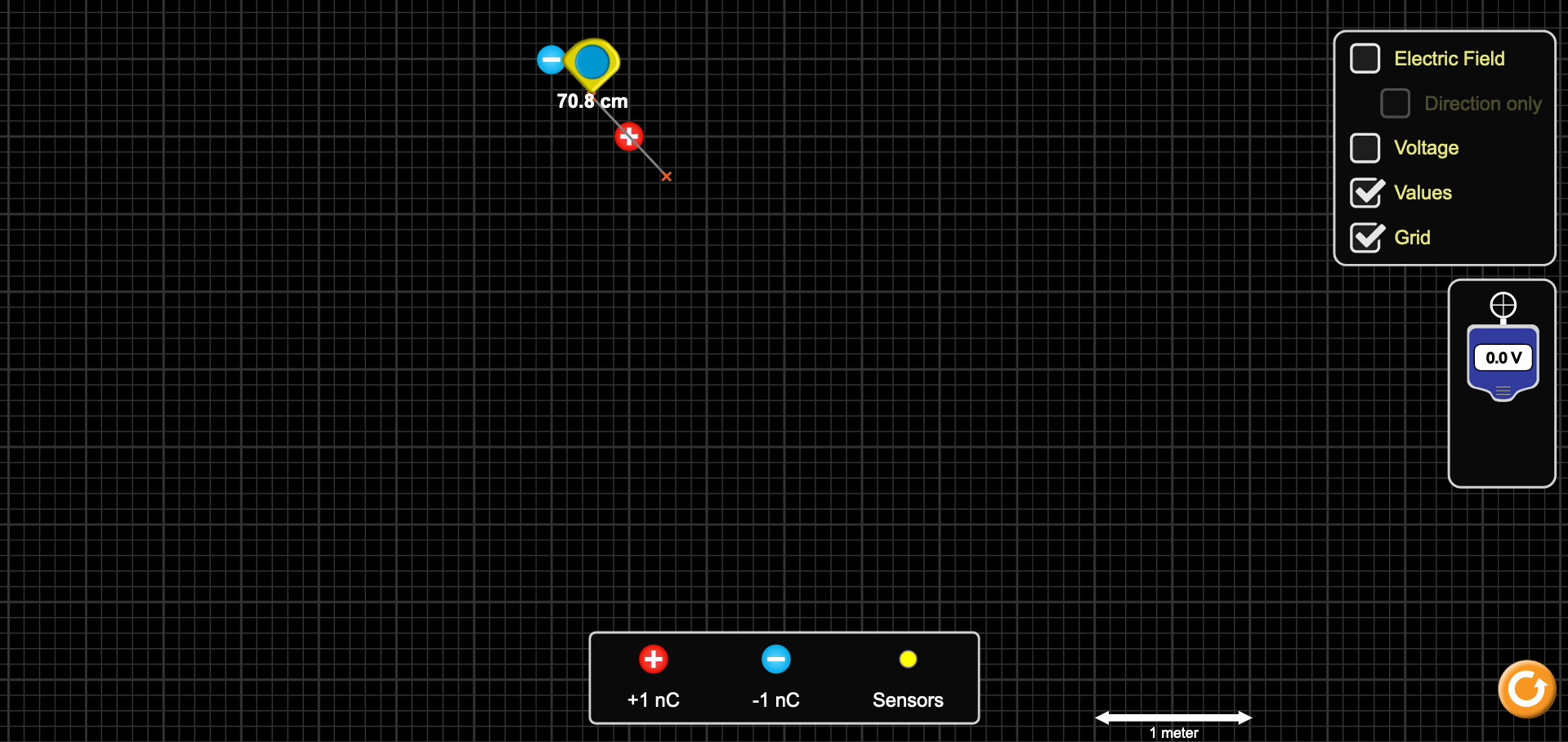
Place one positive and one negative charge into the simulation space, like shown in Figure 3. Note the charges are on corners of one square made by the thick grid lines. Make sure to place the charges somewhere in the upper-left portion of the screen. It is probably also best to have the “Electric Field” and “Voltage” boxes un-checked, so the screen is not too cluttered.

Calculate the separation of the charges, d, using geometry/trigonometry, and report it with its uncertainty in your write up. Use your placement/length uncertainty from the previous section as the uncertainty.

d calculation: 0.5 marks

                                               (a) Location of the first radius

                                              (b) Location of the first radius.

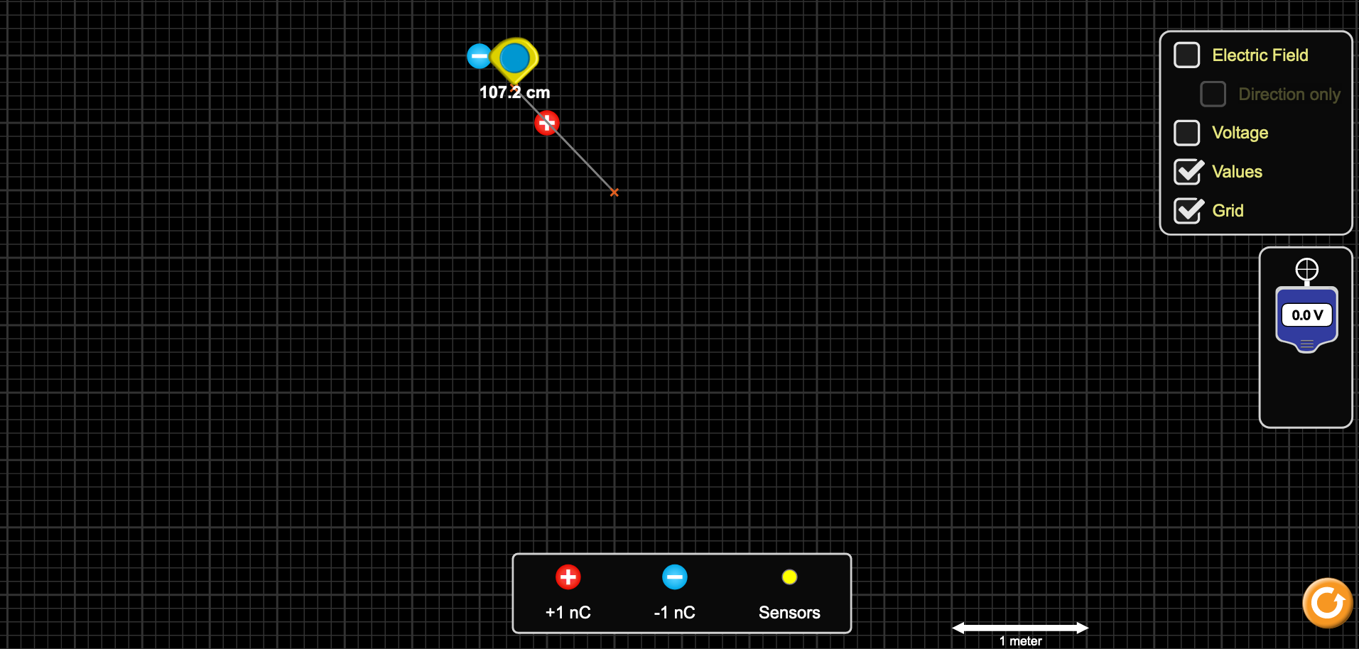
                           Figure 3: Charge and measuring tool setup for θ = 0° measurements.

To measure the first potential, place the distance measuring tool as shown in Figure 3a. One of the orange plus signs should be halfway between the two charges and the other at the point where you want to measure the potential. For the first radius, this point is in the center of the square to the lower-right of the positive charge. The length should be about 0.7 m. Record the length you measure in the first row of the leftmost column (r_0) in Table 3 of the “Theta=0 Table” page of the Capstone workbook. Note that the angle between (the measuring tool line) and the dipole moment vector is zero.

Now take the voltmeter and place the white crosshairs over the orange plus sign where you want to measure the potential. Record the potential from the voltmeter into Table 2a on the “Measurements at Theta=0” page of the Capstone workbook. Put the voltmeter down somewhere away from the charges, then put it back in the same place, and record the value in the next row of Table 2a. Repeat this procedure one more time for this radius, so you have three measurements of the potential at this position.

To measure the second potential, move the second orange plus sign to the bottom-right corner of the (thicker lined) square. Figure 3b shows what this second radius should look like, and the length should now be about 1.06 m. Record the length in the second row in Table 3 (“Theta=0 Table”), measure and record the potential three times in Table 2b, similar to above.

Repeat this procedure seven more times, moving farther away from the dipole, one half of the diagonal distance of a big square at a time, until there are nine entries total for r_0 in Table 3 and Tables 2 are filled in. Each new radius will be half a square farther from the charges than the last one, moving diagonally down and right.

Analysis with θ = 0°

Copy the standard deviation from the “Placement Uncertainty” table (Table 1) into the nine rows of the r_0 column in Table 3. Recall this standard deviation is the uncertainty for all lengths in this experiment. Then copy all the mean and standard deviation voltages from Tables 2 into the Vm_0, Vm_copy and Vm_0 columns respectively, being careful to ensure each voltage lines up with its appropriate corresponding distance. The quantity 1/r_0² and its corresponding uncertainty should now be calculated.

V_m vs. 1/r²

Figure 1 shows the potential you measured (Vm_0) as a function of the quantity 1/r_0². If Equation 3 indeed approximates the measured potential well, then the graph of these two quantities should be a straight line.

Copy your full set of data from Table 3 into Table 4 on the Capstone workbook page “Linear Fit Subset”. On this page, you want to create a subset of your data by removing some data points to see if the linear fit improves. Thinking of your answer to Question 2, try deleting rows of data one at a time and watch how the fit changes. Experiment here a bit. Notice there is an extra column in Table 4: “r_0/d” and consider the discussion from your hypothesis and the introduction section. If you delete more data than you meant to, you can go back and recopy the data from Table 3.

Once you are satisfied that your subset of data is sufficiently well described by a linear fit, we will estimate the uncertainties on the slope and intercept as we have done in the first two experiments. We will use the same method as before, following Section 3.6 in the reference material manual, with the help of the tables and figures in the “Linear Plot Uncertainties” sheet of the data workbook. Include the best-fit-line equation, with uncertainties and proper significant figures, in the associated section of your report. When reporting your final result, please do so as an equation of the form

(1)  

and remember to switch to variables you used in your hypothesis. It is fine to leave off units for values that are not supposed to have units, but make sure to include units if they should be there.

Sample calculation for the linear fit slope and y-intercept uncertainties:

0.75 marks

Report of the linear fit equation: 0.25 marks

V_c / V_m vs. r

Table 6 on the “Compare to Approximation” page in the Capstone workbook shows your data with a few extra values, including: the ratio of the distance from the dipole to the charge separation distance, r_0/d, the (approximate) calculated potential from Equation 3, Vc_0, and the ratio of the measured to theoretical/calculated potential to the measured potential, Vc_0/Vm_0, as well as the corresponding uncertainties.

Figure 4 on the “V_c/V_m Graph” page in the Capstone workbook shows on the y-axis the approximate, calculated potential from Equation 3, , divided by the potentials you measured in the simulation, . On the x-axis we have the radius that you measured each potential at, , divided by the separation between the charges, . The values of the y-axis work like this:

• If the y-value , then .
• If the y-value , then .
• If the y-value , then .

The same is done on the x-axis where we divide your radius by the separation of the charges, . This tells you if your radius is greater than, equal to, or less than the charge separation.

Measuring the dipole potential with θ = 45°

We will now conduct an analogous exercise but in a configuration where the angle between the dipole moment vector and the vector pointing to the position we’re measuring the potential at is . However, we will only take two data points as opposed to nine.

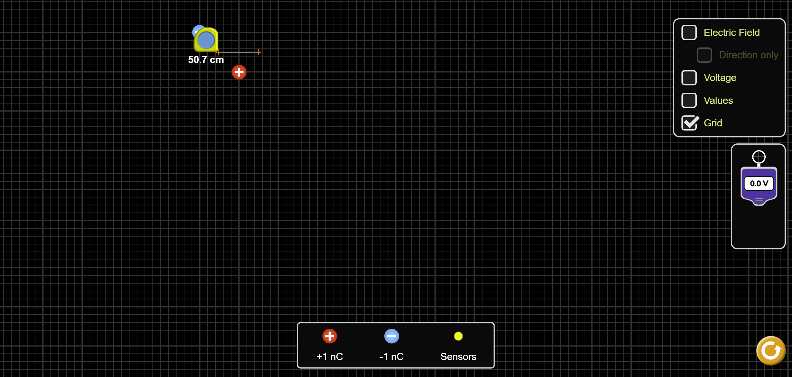
Keep the charges where you left them at the end of Section 2.2. Keep the measuring tool halfway between the two charges, but move the second orange plus sign to the center of the square immediately to the right of the charges. Figure 4a shows what this first radius should look like, and the distance should be about 0.5 m. Notice that the line from the measuring tool makes a 45° angle with the line going from the negative to the positive charge. Record the length in the first row of the leftmost column (for r_45) in Table 8 on the “Theta=45” page, then measure and record the potential three times in Table 7a.

Now move the second orange plus sign seven large squares away to the right. Figure 4b shows what this radius should look like, and the distance should be about 3.75 m. Record your measurement of the length in Table 8 and three measurements of the potential in Table 7b.

Analysis with θ = 45°

As before, copy the standard deviation from the “Placement Uncertainty” table (Table 1) into the first two rows of the _45 column. Then copy all the mean and standard deviation voltages from Tables 7 into the Vm_45 and Vm_45 columns respectively, making sure that each voltage you copy over lines up with its appropriate corresponding distance from the centre of the dipole. All columns in Table 8 (i.e. r_45/d, Vc_45, and Vc_45/Vm_45, as well as their corresponding uncertainties) should then become filled out.

There are no graphs associated with these data. Instead, we will look at values from Table 5 directly.

                                                  (a) Location of the first radius

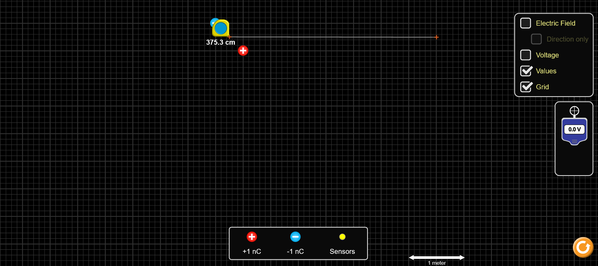
                                               (b) Location of the second radius

              Figure 4: Charge and measuring tool setup for θ = 45° measurements.

Digital submission (2.75 marks total):

Figure 1: 0.5 marks

Figure 2: 0.75 marks

Figure 3: 0.5 marks

Figure 4: 0.5 marks

Capstone Workbook: 0.5 marks

Saving your Capstone workbook

     Here we discuss how and where to store the results from your Capstone workbook for marking. If any of the following instructions are unclear, be sure to double-check that you are doing this correctly with your TA.

     To save your work, we will make use of the “snapshot” feature in the Capstone software.

A snapshot of each page can be recorded with the following steps:

• Click the drop-down arrow next to the camera button near the top of the screen.
• Make sure the “Snapshot Workbook Page Content” option is selected.
• Click the camera button. This will take a snapshot of the current workbook page.

The yellow button to the right of the camera button that looks like a book will display the “Journal,” which is an area within the Capstone software that stores the snapshots as they are taken. This button merely toggles the display of the journal within the software window. All snapshots will be stored to the journal whether this button is active or not. Be sure to check the Journal to ensure you have taken a snapshot of every page of your workbook. Note: This includes the page with your names and student numbers! If you would like to delete a snapshot, you can do so by clicking on the snapshot, then clicking on the red “x” button at the top of the journal window.

When your journal is complete, you are ready to export your snapshots. Export your Journal by finding the icon in the Journal window near the top that looks like a folder with a small arrow pointing to it. If you hover the mouse cursor over the icon but don’t click, it should say “Export to HTML”. Click this button, and be patient if nothing happens immediately–sometimes this action takes several moments. When the software is ready, a File Explorer window will open on the screen, and you will be asked to select a folder to export the Journal to. Navigate to the Desktop, enter the folder that corresponds to your Lab section, and then the workstation number that you are at. Once you have successfully exported your Journal, the File Explorer window will close.

Finally, before you leave the lab, find your exported Journal by opening a new File Explorer window and navigating into the folder/directory that you exported to. You should see a folder with the name of the experiment–specifically, the name of the Capstone software file. Within this folder should be one HTML file and a series of PNG images, one for each of your Capstone workbooks. These images will make up the digital portion of your lab submission. Double check with your TA that your snapshots have been taken properly before you leave.