Mathematical Models
Throughout this discussion, the term “model”, referring to a mathematical model, is used. For the current discussion, a model is defined as a description of the essential features of a system through mathematical equations. It is a representation of a process, system, or behaviour using mathematical language. A simple form of a mathematical model is:
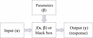
y = f(x, β).
In this example, the goal is to apply a function, f, to some input values x to obtain output values, or responses, denoted as y. The boldface non-italicized x and y indicate that the input and output can consist of multiple values of x and y, respectively. In mathematical terms, these multiple values that constitute a single input is called a vector. Hence, the input to the model is the vector of values. The β (Greek letter “beta”) denotes a vector of parameters, or β values, that are used to transform x into the output of the model. Usually, the parameters are unknown and must be estimated from observations. This process is known as parameter estimation. The response, of the model, y is the result of applying mathematical transformations to the input values x, using the parameters β. The function f may be a simple equation, such as y = f(x) = 2x + β, a set of equations, or a complex black box function that is not well understood. This model is shown graphically below. The function is called “black box” because the internal workings of the model are obscured to the user; that is, the model is metaphorically placed into an opaque black box, hiding computational details.
Realistic models must also account for noise, or randomness, in the model. Such noise is usually denoted by e (Greek letter “epsilon”). Hence, the above model can incorporate the noise term, and is rewritten as:
y = f(x, β) + ε.
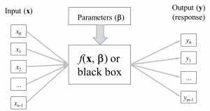
As mentioned, models can have multiple inputs, but can also have multiple responses. The model below represents a model with n inputs – that is, each input vector, x, consists of n values of x, and m outputs; that is, each output vector, y, consists of m values of y.
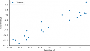
Linear regression is a simple linear model used to model the relationship between explanatory variables (the input, or predictors) and observed values (the response). The goal is to determine the parameters of the linear model to minimize the error between the observed values and those predicted by the model. For instance, suppose that the following responses were observed for different values of the explanatory variable. The situation can be visualized as a scatter plot, as shown below. Note that there is some noise present in the observed values, which is the reason that they do not lie on a straight line.
The goal is to determine a best-fit line through these observations that minimizes the difference between the observed values and the values obtained from the equation of the model that is being determined. A line is modeled as y = ax + b, where a is the slope of the line, and b is the y-intercept, where the line crosses the y-axis. Performing a linear regression on the predictor-response pairs yields the following result, shown below.
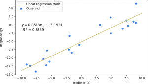
In this example, the parameters a (slope) and b (y-intercept) were determined to be 0.8588 and -5.1921, respectively. The coefficient of determination, R2, indicates how well the parameters produce a line that models the observed data. R2 values close to 1.0 indicate a good fit. In this example, R2 = 0.8839, indicating that the parameters model the observed values well.
