Applications Of N-Grams
Cultural Trends
One of the first applications of n-grams was research into cultural trends through the large-scale analysis of printed material from a large corpus from over five million books obtained from the Google Books project. The work was performed by a collaborative team of researchers from Harvard University, Google, and elsewhere. The corpus contains over 500 billion words in seven languages – English, German, Hebrew, Chinese, French, Spanish, and Russian.
Subsequent analysis was performed on the resulting n-grams. The mean percentages of overall frequency for words and phrases by year, based on different criteria were computed and used in subsequent statistical analysis. The authors demonstrated this approach with the word “treaty”. The mean percentage of overall frequency against time (increasing years), relative to treaty signature, was plotted and analyzed. The same approach was used to analyze heads of state relative to their accession to power, as well as changes in the names of countries over time (Michel et al., 2011).
Word Usage in Novels and Published Literature
In the article Digital Humanities, Big Data, and Ngrams, University of California, Berkeley sociologist Claude S. Fischer reports on some recent studies, including one by historian Marc Egnal analyzing the evolution of the American novel (Egnal, 2013), employing n-grams to research into the dynamic (time-varying) patterns of word usage and how they are reflected in cultural trends.
Some interesting findings are that the word “gentleman” appears approximately 130 times more than the word “guy” in books from the early part of the twentieth century. By 2000, however, there was a shift: the word “gentleman” was only used about one-third as often as “guy”. Another observation was that the word “I” at the start of a sentence, indicating the subject of the ensuing action, was about 70% of that of the words “He” or “She” in both 1970 and 2000. However, there was a drop in the ratio of “I” to “You” at the start of a sentence over the same period, possibly indicating that “I-absorption” is not as common as previously thought. Additionally, the word “vampire” occurs about 10 times more frequently in 2008 than in 1950, the cultural implications of which Fischer leaves open.
However, as Fischer points out, n-gram analysis comes with some challenges. First, there is the issue of which material to use. This human curation of sources, as explained in earlier sections, always involves a subjective element. Beyond curation, the books that survived, and therefore could be scanned and subjected to quantitative analysis, are not the entirety of books that were published. As a large component of the material scanned by the Google Books project is contributed from libraries, the curation of those library materials affects the results of any n-gram analysis. For instance, many libraries did not acquire books that contain crude language or obscenities, and therefore, those books cannot be scanned and analyzed, further problematizing n-gram interpretation. Consequently, many factors contribute to which books survived, and, of those, which books were ultimately selected for further investigation. Furthermore, as Fischer points out, the volume and types of books that were published varies greatly over time. Early in the history of the U.S., for instance, books were very expensive to print, and did not have a widespread readership. During the early periods, books were mostly didactic in nature. It was only later that romance and adventure novels became popular with a corresponding change in the mixture of words that were used in these books.
Another interesting complicating factor in n-gram analysis is the size of the vocabulary. In 1950, for instance, approximately 597,000 words were included in the English lexicon, whereas this number increased to 1,022,000 in 2000, an increase of 71%, or about 1.4% per year on average. The introduction of new words into the lexicon displaces many words that were more common in earlier times. Despite the increase in the size of the lexicon, in the United States, a decrease in the size of the vocabulary used by the population was observed, and therefore the words in popular usage changed accordingly. Furthermore, word meanings shift over time. For instance, the word “text”, in addition to its standard definition, has recently also been gaining usage as a verb and therefore drawing semantic conclusions based strictly on n-grams may be problematic.
N-gram Visualization Example
The following example is an adaptation of a procedure found in:
Ednalyn C. De Dios
May 22, 2020
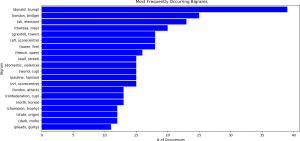
In the following example, bigrams (2-grams) were calculated for news headlines from the ABC (Australian Broadcasting Company) website. The data were obtained from [Here]. Daily headline text is reported for the period from February 2003 through June 2017, but, for illustrative purposes, the data were combined on a monthly basis. That is, all the headline text for each day in a particular month was aggregated into one large text string, which was subsequently processed with the Python NLTK (Natural Language Toolkit) library. (Note: The entire procedure for performing this analysis is explained and demonstrated in a subsequent course.) The top 50 unigrams, bigrams, and trigrams were then calculated for each month in each year. These n-grams can be represented in a horizontal bar charts, as shown below. For clarity, only the top 20 unigrams, bigrams, and trigrams are displayed.
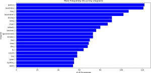
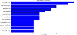
Note that the frequencies, or numbers of occurrences, for trigrams are much smaller than that for unigrams, and that there is less variation in the counts from unigrams to trigrams.
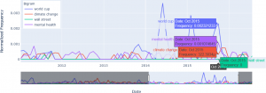
Although this chart provides useful information (e.g. that the bigrams for “Donald Trump”, “London Bridge”, and “UK Election” are the most frequent over the entire time period), analyzing the bigram dynamics – that is, how the frequencies change over time – is usually more important, as described in the more detail below. Dynamic n-grams can be displayed as a line chart using an interactive plotting library (the Plotly library in Python for this example) to facilitate analysis at different resolutions and time periods. For instance, suppose that a researcher needs to analyze and compare the bigrams for “World Cup”, “Climate Change”, “Wall Street”, and “Mental Health”, to examine correlations, for example. The ABC News headlines can be analyzed in this way through bigrams. A plot of the interactive bigram display is shown below for these four bigrams. A time selector below the plot allows the user to more closely examine a shorter time period – that is, to “zoom in”. The values on the y-axis are normalized frequency values. The counts for each n-gram for time t are divided by the number of words in the corpus for time t. This normalization procedure prevents n-grams that appear in small texts being assigned disproportionately high weights.
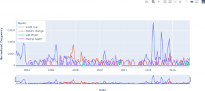
The plot below shows the result limiting the time window to the period from January 2011 to August 2016. The plot allows the user to hover over a time series of interest, and, using the “Compare data on hover” feature in Plotly, the individual frequencies for the four bigrams are displayed.
Google Ngram Viewer
The Ngram Viewer by Google, also known as the Google Books Ngram Viewer, is an online query-based tool, search engine, and visualization system that displays graphs for the frequencies of words, terms, or phrases. Specifically, it employs an annual aggregate of n-grams determined from printed material between 1500 and 2019 (as of November 13, 2021). The English, Chinese, French, German, Hebrew, Italian, Russian, and Spanish languages are supported. Ngram Viewer was developed as a tool to support the Google Books initiative, currently the largest digitized collection of books. It is widely used in a variety of research projects. The results are displayed as line graphs, with relative frequency (percentage) of the term for each year on the y-axis, and the year on the x-axis, similar to the line graphs in the previous section. Users select the date range to examine (the default is 1800-2019), the language, whether the search is case sensitive, and smoothing.
Smoothing is the process of averaging n-gram counts over a time window. Such averaging is a “smoothing” operation, as sharp differences between frequencies in the time window are attenuated, on average. For instance, a smoothing value of 1 indicates that the frequency for a specific year is calculated as the average of the frequencies for the year prior, the specific year, and the following year. For the year 1988, this means that the frequencies for 1987, 1988, and 1989 are averaged. For a smoothing value of 3, the frequencies for 1985, 1986, 1987, 1988, 1989, 1990, and 1991 will be averaged. In general, for a smoothing value of n, the frequencies in the 2n + 1 time window (n years before the selected year, n years after) centered at the selected year are averaged. The user then inputs one or more entries (words, terms, or phrases) on which to search, separating each separate entry with a comma. The example on the Ngram Viewer main page defaults to the three terms “Albert Einstein”, “Sherlock Holmes”, and “Frankenstein” (November 13, 2021). The three-line graphs are plotted in different colours on the same plot. The user can hover over the plot to view the n-gram percentages displayed simultaneously for the three separate terms for a specific year, normalized by the number of terms represented in that year to enable comparisons of years that have varying numbers of published books. The percentages represent the frequency of the word or term in the entire corpus, calculated as the number of times the term occurs divided by the total number of terms in a specific year. Ngram Viewer supports unigrams, digrams, trigrams, 4-grams, and 5-grams.
The Ngram Viewer also supports wild card searches with the (*) symbol. This feature displays the top ten substitutions for the wild card character. Shai Ophir, in the web article Big Data for the Humanities Using Google Ngrams. Discovering Hidden Patterns of Conceptual Trends demonstrates how iteratively refined wild card queries can be used for uncovering patterns and trends that may not be immediately evident. He provides an example of using the wild card feature for more complex analyses of the word “Truth”. A single wild card entry “Truth *” returns results that may not be meaningful or interesting.
For instance, “Truth and” was the top-ranked bigram, based on the probability of these words occurring together. In an iterative fashion, another search can be performed with “Truth and *”, i.e., substituting the first * with the top-ranking word, and then continuing the query with another wild card search. The new set of top-ranking terms provide some indication of the words that most frequently occur with “Truth”. However, the analysis must proceed further, and “Truth” is subsequently compared with the highest-ranking adjacent words to observer correlations between those words and “Truth”. Continuing the analysis, the time range of the query can be expanded to cover the full range of years supported by Ngram Viewer – over 500 years. Fluctuations in the use of these terms is necessary, as assessing the correlation of the terms is dependent on similar patterns of fluctuation. However, the task is challenging due to the normalization by year. Removing less correlated terms from the queries can be performed to assess correlations in fluctuations. In the example presented by Ophir, this step left the words “Truth”, “Justice”, and “Love”. Inspecting the results reveal the “Love” is most closely correlated with “Truth”, and that “Justice” is correlated with both those words. Additionally, in examining the fluctuations, it was seen that in the mid-1600s, “Truth”, “Justice”, and “Love” increase in frequency, declining at the end of the 1700s. Once interesting fluctuations, such as inclines or declines, are found, a wild card query is again employed to determine other terms that are associated with these fluctuations for specific time periods. In the example, the n-gram percentages for both “Truth” and “Love” increase from 1680-1700, and consequently, the wild card search “Truth *” and “Love *” can be applied to this limited time frame. The top two combinations are determined (in this case, “Truth of” and “Love of”), and the analysis continues in this iterative manner, successively refining the search terms and assessing correlations for the new results that are returned. The result of this analysis is that new patterns for “Truth” were determined, indicating that “Love” is correlated with both “Truth” and “Justice” when correlations were examined for short periods of time – that is, in high level resolution. This example provides a demonstration that Ngram Viewer, when used with carefully constructed queries with the wild card feature, combined with human analysis, can potentially uncover hidden patterns of conceptual trends.
In addition to providing new insights into large corpora of texts, the Ngram Viewer poses some challenges to researchers (Younes & Reips, 2019), especially when studying languages or testing linguistic theories. An issue that must be taken into consideration when performing research with Ngram Viewer, and n-grams in general, is that because the results are based on probabilities, important outliers or meaningful exceptions are sometimes overlooked, especially when querying with the wild card.
On a technical level, Ngram Viewer has been criticized because of its reliance on inaccurate optical character recognition (OCR), which can potentially introduce bias into the results. For instance, OCR was in some cases unable to distinguish between the letters “s” and “f”, whose appearance was very similar before the 1800s (Younes & Reips, 2019). Incorrect OCR also introduces noise into the n-grams, with a consequent negative impact on the statistics. Some languages, such as Chinese, are particularly susceptible to inaccuracies due to OCR problems and a relatively small number of texts.
Another challenge is the uneven distribution of content in the corpora. Scientific literature is particularly over-represented, thereby decreasing the percentage for words outside this domain. Text are also not controlled for bias, and many texts have inaccurate dates or are incorrectly categorized. A further complicating factor is the absence of metadata, and therefore dynamics in linguistics or culture are difficult to assess.
To address these challenges, some guidelines have been proposed, especially for assessing the influences of censorship and propaganda, to test theories or hypotheses, and for cross-cultural examination of results (Younes & Reips, 2019). First, corpora from different languages should be used. Second, although it may initially appear as counterintuitive, using the English (British and American) language fiction corpus (a specialized English language corpus within the Ngram Viewer system) is recommended, as this corpus is less affected by the high volume of scientific literature generally evident throughout the corpora. Third, comparing frequencies of words, as well as their inflections, should be used with the “_INF” tag, causing Ngram Viewer to provide graphs of all available inflections of a specific word. Fourth, researchers should employ synonyms to reduce the risk of inaccuracies due to OCR error or the disproportionately large influence of the contributions of a single authors. Fifth, a standardization procedure is recommended to address variations in the volume of data and uneven weights for words. This standardization can be achieved through z-scoring. A z-score zt is defined as zt = (wt – m) / s, where wt denotes the frequency of word w in year t, and m and s are the mean and standard deviation of wt, respectively. The recommended approach is to subtract the summed z-scores of the frequencies of common words from the summed z-scores of the frequencies of the original terms. The effect is that the disproportionately high influence of a single word is reduced because each of the original terms have equal weight through standardization. Multiple common words can also be investigated in this way. As the set of common words are z-scored, all those words are treated equally (Younes & Reips, 2019).
Google Ngram Viewer provides multifaceted benefits to scholars and scholarship, and has proven to be valuable in studies on gender differences, personality, education, the development of individualism and collectivism, and a host of other topics (Younes & Reips, 2019). Although researchers need to be aware of the challenges that arise when using Ngram results and the limitations inherent in this approach, they may consider employing the guidelines to mitigate these problems and to enhance the accuracy and reliability of the results obtained from Ngram Viewer (Younes & Reips, 2019).
