2.11: Implicit Differentiation and Related Rates
Implicit Differentiation
In our work up until now, the functions we needed to differentiate were either given explicitly, such as [latex]y=x^2+e^x[/latex], or it was possible to get an explicit formula for them, such as solving [latex]y^3-3x^2=5[/latex] to get [latex]y=\sqrt[3]{5+3x^2}[/latex]. Sometimes, however, we will have an equation relating [latex]x[/latex] and [latex]y[/latex] which is either difficult or impossible to solve explicitly for [latex]y[/latex], such as [latex]y+e^y=x^2[/latex]. In any case, we can still find [latex]y' = f'(x)[/latex] by using implicit differentiation.
The key idea behind implicit differentiation is to assume that [latex]y[/latex] is a function of [latex]x[/latex] even if we cannot explicitly solve for [latex]y[/latex]. This assumption does not require any work, but we need to be very careful to treat [latex]y[/latex] as a function when we differentiate and to use the Chain Rule.
Video Demonstration
Implicit Differentiation
© 2014 Eric Bancroft
Example 1
Assume that [latex]y[/latex] is a function of [latex]x[/latex]. Calculate
a. [latex]\frac{d}{dx}\left( y^3 \right)[/latex]
b. [latex]\frac{d}{dx}\left( x^3y^2 \right)[/latex]
c. [latex]\frac{d}{dx}\left( \ln(y) \right)[/latex]
Answer:
a. [latex]\frac{d}{dx}\left( y^3 \right)=?[/latex]
Since [latex]y[/latex] is considered to be a function of [latex]x[/latex], we have that
[latex]y^3=\overbrace{({y(x)})^3}^{composition}=\overbrace{(\text{something involving }x)^3}^{composition}[/latex]
Thus we will need the chain rule since [latex]y^3[/latex] is a power function applied to another (unknown) function of [latex]x[/latex], i.e., a composition of functions.
[latex]\frac{d}{dx}\left( y^3 \right)=\overset{out'}{3y^2}\cdot\overset{in'}{\frac{dy}{dx}}\overset{or}{=}3y^2y'[/latex]
b. [latex]\frac{d}{dx}\left( x^3y^2 \right)=?[/latex]
Let's analyze the function:
[latex]x^3y^2=\overbrace{x^3\cdot \overbrace{(y(x))^2}^{composition}}^{product}[/latex]
Therefore we need to use the product rule and the chain rule:
[latex]\begin{align*} \frac{d}{dx}\left( x^3y^2 \right) & = \overset{first'}{3x^2}\cdot \overset{second}{\overset{}{y^2}}+\overset{first}{\overset{}{x^3}}\cdot\overset{second'}{\underset{out'}{\underset{}{2y}}\cdot\underset{in'}{\underset{}{\frac{dy}{dx}}} }\\ & = 3x^2y^2+2x^3y\frac{dy}{dx} \\\\ &\overset{\text{or}}{=} 3x^2y^2+2x^3yy' \end{align*}[/latex]
c. [latex]\frac{d}{dx}\left( \ln(y) \right)=?[/latex]
Since [latex]\ln(y)=\ln(y(x))[/latex], this is a composition of functions with no other operations and so we simply apply the chain rule:
[latex]\frac{d}{dx}\left( \ln(y) \right)=\frac{1}{y}\cdot \frac{dy}{dx}=\frac{1}{y}\cdot y'[/latex]
To determine [latex]y'[/latex], differentiate each side of the defining equation, treating [latex]y[/latex] as a function of [latex]x[/latex], and then algebraically solve for [latex]y'[/latex].
Video Demonstration
Implicit Differentiation - more examples
© 2014 Eric Bancroft
(The last example in the following video gets rather messy - don't worry too much if you can't follow all of the simplifications at the end.)
Video Demonstration
Implicit Differentiation - and more examples
© 2014 Eric Bancroft
Example 2
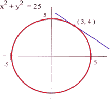
Find the slope of the tangent line to the circle [latex]x^2 + y^2 = 25[/latex] at the point (3, 4) using implicit differentiation.
Answer: The slope of the tangent line will be equal to [latex]\frac{dy}{dx}[/latex] evaluated at the point (3, 4).
We differentiate each side of the equation [latex]x^2 + y^2 = 25[/latex] and then solve for [latex]y'[/latex]:
[latex]\begin{align*} & x^2 + y^2 = 25\\\\ \Rightarrow\quad &\frac{d}{dx}\left(x^2+y^2\right) = \frac{d}{dx}(25)\\\\ \Rightarrow\quad & 2x+2yy' = 0\\\\ \Rightarrow\quad & 2yy'=-2x\\\\ \Rightarrow\quad & y'=-\frac{x}{y} \end{align*}[/latex]
Therefore, at the point (3,4), [latex]y'=-\frac{3}{4}[/latex] and so slope of the tangent line at (3, 4) is 0.75.
Here is a visual representation:
Example 3
Suppose that the price-demand for a product can be described using
[latex]p=0.05x^{3}-0.2x^{2}+0.5[/latex]
where [latex]x[/latex] is the daily demand (in thousands) and [latex]p[/latex] is unit price (in $). Determine the rate of change in demand when price is $1.50 per unit and interpret your result.
Answer: [latex]dx/dp=?[/latex] when [latex]p=1.50[/latex], interpretation?
The price-demand equation cannot be (easily) solved for [latex]x[/latex], so we will use implicit differentiation.
[latex]\begin{align*} & p=0.05x^{3}-0.2x^{2}+0.5\\\\ \Rightarrow\quad &\frac{d}{dp}(p)=\frac{d}{dp}\left(0.05x^{3}-0.2x^{2}+0.5\right)\\\\ \Rightarrow\quad &1=0.15x^2\frac{dx}{dp}-0.4x\frac{dx}{dp}+0\\\\ \Rightarrow\quad &1=(0.15x^2-0.4x)\frac{dx}{dp}\\\\ \Rightarrow\quad &\frac{dx}{dp}=\frac{1}{0.15x^2-0.4x} \end{align*}[/latex]
At [latex]p=1.50[/latex], we have
[latex]\dfrac{dx}{dp}=\frac{1}{0.15x^2-0.4x}=\frac{1}{0.15(1.5)^2-0.4(1.5)}\approx 3.8[/latex]
and so at $1.50 per unit, the demand is decreasing by approximately 3,800 units per $1 increase in price, or by approximately 380 units per $0.10 increase in price.
Video Demonstration
Equation of the tangent line using implicit differentiation
© 2014 Eric Bancroft
Related Rates
If several variables or quantities are related to each other and some of the variables are changing at a known rate, then we can use derivatives to determine how rapidly the other variables must be changing.
Here is a link to the examples used in the videos in this section: Related Rates.
Video Demonstration
Related Rates - Example 1
© 2014 Eric Bancroft
Example 4
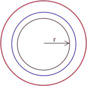
Suppose the border of a town is roughly circular, and the radius of that circle has been increasing at a rate of 0.1 miles each year. Find how fast the area of the town has been increasing when the radius is 5 miles.
Answer:
We could get an approximate answer by calculating the area of the circle when the radius is 5 miles ([latex]A = \pi r^2 = \pi (5 \text{ miles})^2 \approx 78.6 \text{ miles}^2[/latex] ) and 1 year later when the radius is 0.1 feet larger than before ([latex]A = \pi r^2 = \pi (5.1 \text{ miles})^2 \approx 81.7 \text{ miles}^2[/latex] ) and then finding [latex]\frac{\Delta \text{Area}}{\Delta \text{time}}=\frac{81.7 \text{ mi}^2 - 78.6 \text{ mi}^2}{1 \text{ year}} = 3.1 \text{ mi}^2/\text{yr}.[/latex] This approximate answer represents the average change in area during the 1 year period when the radius increased from 5 miles to 5.1 miles, and would correspond to the secant slope on the area graph.
To find the exact answer, though, we need derivatives. In this case both radius and area are functions of time: [latex]r(t)=\text{ radius at time } t \qquad A(t)=\text{ area at time } t[/latex]
We know how fast the radius is changing, which is a statement about the derivative: [latex]\frac{dr}{dt}=0.1\frac{\text{mile}}{\text{year}}[/latex]. We also know that [latex]r = 5[/latex] at our moment of interest.
We are looking for how fast the area is increasing, which is [latex]\frac{dA}{dt}[/latex].
Now we need an equation relating our variables, which is the area equation: [latex]A=\pi r^2.[/latex]
Taking the derivative of both sides of that equation with respect to [latex]t[/latex], we can use implicit differentiation:
[latex]\begin{align*} \frac{d}{dt}\left( A \right) & = \frac{d}{dt}\left( \pi r^2 \right)\\ \frac{dA}{dt} & = \pi 2r\frac{dr}{dt} \end{align*}[/latex]
Plugging in the values we know for [latex]r[/latex] and [latex]\frac{dr}{dt}[/latex], [latex]\frac{dA}{dt}=\pi 2(5\text{ miles})\left(0.1\frac{\text{miles}}{\text{year}}\right)=\pi\frac{\text{miles}^2}{\text{year}}[/latex]
So the area of the town is increasing by approximately 3.14 square miles per year when the radius is 5 miles.
Related Rates
When working with a related rates problem,
- Draw a picture (if possible).
- Identify the quantities that are changing, and assign them variables.
- Find an equation that relates those quantities.
- Differentiate both sides of that equation with respect to time.
- Plug in any known values for the variables or rates of change.
- Solve for the desired rate.
Example 5
A company has determined the demand curve for their product is [latex]q=\sqrt{5000-p^2}[/latex], where [latex]p[/latex] is the price in dollars, and [latex]q[/latex] is the quantity in millions. If weather conditions are driving the price up $2 a week, find the rate at which demand is changing when the price is $40.
Answer:
The quantities changing are [latex]p[/latex] and [latex]q[/latex], and we assume they are both functions of time, [latex]t[/latex], in weeks. We already have an equation relating the quantities, so we can implicitly differentiate it.
[latex]\begin{align*} \frac{d}{dt}(q) & = \frac{d}{dt}\left(5000-p^2\right)^{1/2} \\ \frac{dq}{dt} & = \frac{1}{2}\left(5000-p^2\right)^{-1/2}\frac{d}{dt}\left(5000-p^2\right) \\ \frac{dq}{dt} & = \frac{1}{2}\left(5000-p^2\right)^{-1/2}\left(-2p\frac{dp}{dt}\right) \end{align*}[/latex]
Using the given information, we know the price is increasing by $2 per week when the price is $40, giving [latex]\frac{dp}{dt}=2[/latex] when [latex]p = 40[/latex]. Plugging in these values,
[latex]\frac{dq}{dt} = \frac{1}{2}\left(5000-40^2\right)^{-1/2}\left(-2(40)(2)\right) \approx -1.37[/latex]
Demand is falling by 1.37 million items per week.
Example 6
The total daily cost for producing [latex]x[/latex] items in a day is [latex]TC(x) = 300,000 + 4x + \frac{200,000}{x}[/latex]. If production has been ramping up by 20 items a day, find the rate at which total daily cost is increasing, if they are currently producing 2,000 items.
Answer:
The quantities changing are [latex]x[/latex] and [latex]TC[/latex], and we assume they are both functions of time, [latex]t[/latex], in days. We already have an equation relating the quantities, so we can implicitly differentiate it.
[latex]\begin{align*} \frac{d}{dt}(TC) & = \frac{d}{dt}\left(300,000 + 4x + 200,000x^{-1}\right) \\ \frac{d TC}{dt} & = 4\frac{dx}{dt} - 200,000x^(-2)\frac{dx}{dt}\\ \frac{d TC}{dt} & = \left(4 - \frac{200,000}{5000^2}\right)\frac{dx}{dt}\\ \end{align*}[/latex]
We know the quantity produced is increasing by 20 items per week when the production is 2,000 items, giving [latex]\frac{dx}{dt}=20[/latex] when [latex]x = 2000[/latex]. Plugging in these values,
[latex]\frac{d TC}{dt} = \left(4 - \frac{200,000}{2000^2}\right)(20) = 79[/latex]
Total daily cost is increasing by $79 each day.
Section Exercises
Work on the following exercises. Discuss your solutions with your peers and/or course instructor.
MA4B Exercises 2.11 - Implicit Differentiation and Related Rates
