2.3 The Basic Rules for Derivatives
In the next few sections, we’ll get the derivative rules that will let us find formulas for derivatives when our function comes to us as a formula. This is a very algebraic section, and you should get lots of practice. When you tell someone you have studied calculus, this is the one skill they will expect you to have.
Video Demonstration
Introduction to derivatives of formulas
© 2014 Eric Bancroft
Building Blocks
These are the simplest rules – rules for the basic functions. We won’t prove these rules; we’ll just use them. But first, let’s look at a few so that we can see they make sense.
Example 1
Find the derivative of [latex]y=f(x)=mx+b[/latex]
Answer:
This is a linear function, so its graph is its own tangent line! The slope of the tangent line, the derivative, is the slope of the line: \[f'(x)=m\]
Linear Function Rule:
Video Demonstration
Slope of a linear function
© 2014 Eric Bancroft
Example 2
Find the derivative of [latex]f(x)=135[/latex].
Answer:
Think about this one graphically, too. The graph of f(x) is a horizontal line. So its slope is zero: \[f'(x)=0\]
Constant Function Rule:
Video Demonstration
Slope of a constant function
© 2014 Eric Bancroft
Example 3
Find the derivative of [latex]f(x)=x^2[/latex].
Answer:
Recall the formal definition of the derivative: \[f'(x)=\lim\limits_{h\to 0} \frac{f(x+h)-f(x)}{h}.\]Using our function [latex]f(x)=x^2[/latex], [latex]f(x+h)=(x+h)^2=x^2+2xh+h^2[/latex].
Then
\[ \begin{align*}
f'(x) & = \lim\limits_{h\to 0} \frac{f(x+h)-f(x)}{h}\\
& = \lim\limits_{h\to 0} \frac{x^2+2xh+h^2-x^2}{h}\\
& = \lim\limits_{h\to 0} \frac{2xh+h^2}{h}\\
& = \lim\limits_{h\to 0} \frac{h(2x+h)}{h}\\
& = \lim\limits_{h\to 0} (2x+h)\\
& = 2x
\end{align*} \]
From all that, we find that [latex]f'(x)=2x[/latex].
Luckily, there is a handy rule we use to skip using the limit:
Power Rule
Video Demonstration
Power rule – example 1; Power rule – example 2
© 2014 Eric Bancroft
Example 4
Find the derivative of [latex]g(x)=4x^3[/latex]
Answer:
Using the power rule, we know that if [latex]f(x)=x^3[/latex], then [latex]f'(x)=3x^2[/latex]. Notice that [latex]g[/latex] is 4 times the function [latex]f[/latex]. Think about what this change means to the graph of [latex]g[/latex] – it’s now 4 times as tall as the graph of [latex]f[/latex]. If we find the slope of a secant line, it will be [latex]\frac{\Delta g}{\Delta x}= \frac{4\Delta f}{\Delta x} =4\frac{\Delta f}{\Delta x}[/latex]; each slope will be 4 times the slope of the secant line on the [latex]f[/latex] graph. This property will hold for the slopes of tangent lines, too: \[\frac{d}{dx}\left(4x^3\right)=4\frac{d}{dx}\left(x^3\right)=4\cdot 3x^2=12x^2.\]
Constant Multiple Rule:
Video Demonstration
Constant multiples of functions
© 2014 Eric Bancroft
Here are all the basic rules in one place.
Derivative Rules: Building Blocks
In what follows, [latex]f[/latex] and [latex]g[/latex] are differentiable functions of [latex]x[/latex].
Constant Multiple Rule
\[ \frac{d}{dx}\left( kf\right)=kf’\]
Sum and Difference Rule
\[\frac{d}{dx}\left(f\pm g\right)=f’ \pm g’\]
Power Rule
\[\frac{d}{dx}\left(x^n\right)=nx^{n-1}\]
Special cases:
\[\frac{d}{dx}\left(k\right)=0 \quad \text{because }[latex]k=kx^0[/latex]\].
\[\frac{d}{dx}\left(x\right)=1 \quad \text{because } [latex]x=x^1[/latex]\]
Exponential Functions
\[\frac{d}{dx}\left(e^x\right)=e^x\] \[\frac{d}{dx}\left(a^x\right)=\ln(a)\,a^x\]
Natural Logarithm
\[\frac{d}{dx}\left(\ln(x)\right)=\frac{1}{x}\]
The sum, difference, and constant multiple rules combined with the power rule allow us to easily find the derivative of any polynomial.
Video Demonstration
Sum and difference of functions; Exponential function and natural log
© 2014 Eric Bancroft
Example 5
Find the derivative of [latex]p(x)=17x^{10}+13x^8-1.8x+1003[/latex].
Answer:
\[
\begin{align*}
&\frac{d}{dx}\left( 17x^{10}+13x^8-1.8x+1003 \right) \\\\
& =\frac{d}{dx}\left( 17x^{10} \right)+\frac{d}{dx}\left( 13x^8 \right)-\frac{d}{dx}\left( 1.8x \right)+\frac{d}{dx}\left( 1003 \right)\\\\
& = 17\frac{d}{dx}\left( x^{10} \right)+13\frac{d}{dx}\left( x^8 \right)-1.8\frac{d}{dx}\left( x \right)+\frac{d}{dx}\left( 1003 \right)\\\\
& = 17\left(10x^9\right)+13\left(8x^7\right)-1.8\left(1\right)+0\\\\
& = 170x^9+104x^7-1.8
\end{align*}
\]
You don’t have to show every single step. Do be careful when you’re first working with the rules, but pretty soon you’ll be able to just write down the derivative directly:
Example 6
Find [latex]\frac{d}{dx}\left( 17x^2-33x+12 \right)[/latex].
Answer:
Writing out the rules, we’d write \[\frac{d}{dx}\left( 17x^2-33x+12 \right)=17(2x)-33(1)+0=34x-33.\]
Once you’re familiar with the rules, you can, in your head, multiply the 2 times the 17 and the 33 times 1, and just write \[\frac{d}{dx}\left( 17x^2-33x+12 \right)=34x-33.\]
The power rule works even if the power is negative or a fraction. In order to apply it, first translate all roots and basic rational expressions into exponents:
Example 7
Find the derivative of [latex]y=3\sqrt{t}-\frac{4}{t^4}+5e^t[/latex].
Answer:
The first step is translate into exponents: \[y=3\sqrt{t}-\frac{4}{t^4}+5e^t=3t^{1/2}-4t^{-4}+5e^t\]
Now you can take the derivative:
\[ \begin{align*}
\frac{d}{dt}\left( 3t^{1/2}-4t^{-4}+5e^t \right) & = 3\left(\frac{1}{2}t^{-1/2}\right)-4\left(-4t^{-5}\right)+5\left(e^t\right) \\
& = \frac{3}{2}t^{-1/2}+16t^{-5}+5e^t
\end{align*} \]
If there is a reason to, you can rewrite the answer with radicals and positive exponents: \[y’= \frac{3}{2}t^{-1/2}+16t^{-5}+5e^t= \frac{3}{2\sqrt{t}}+\frac{16}{t^5}+5e^t\]
Be careful when finding the derivatives with negative exponents.
We can immediately apply these rules to solve the problem we started the chapter with – finding a tangent line.
Example 8
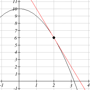
Find the equation of the line tangent to [latex]g(t)=10-t^2[/latex] when [latex]t = 2[/latex].
Answer: Recall that the tangent of a function at a particular input value is the line sharing the point and the slope with the function at that input value. So the equation of the tangent to [latex]g(t)[/latex] at [latex]t=2[/latex] has the form [latex]y=mt+b[/latex], where [latex]m[/latex] is the derivative of [latex]g[/latex] at [latex]t=2[/latex] and the line passes through the point [latex](2, g(2))[/latex].
Since the slope of the tangent line is the value of the derivative, we have [latex]g'(t)=-2t[/latex] and so [latex]m=g'(2)=-4[/latex].
Therefore, the tangent equation is [latex]y=-4t+b[/latex].
We still have to determine the value of [latex]b[/latex]. Since the tangent line touches the original function at [latex]t = 2[/latex], we can find the point by evaluating the original function: [latex]g(2)=10-2^2=6[/latex]. The tangent line must pass through the point (2, 6).
By substituting the coordinates into the equation of the tangent, we get
[latex]6=-4(2)+b\Rightarrow b=6+4(2)=14[/latex]
Therefore, the equation of the tangent is [latex]y=-4t+14[/latex].
Graphing, we can verify this line is indeed tangent to the curve:
We can also use these rules to help us find the derivatives we need to interpret the behavior of a function.
Example 9
In a memory experiment, a researcher asks the subject to memorize as many words from a list as possible in 10 seconds. Recall is tested, then the subject is given 10 more seconds to study, and so on. Suppose the number of words remembered after [latex]t[/latex] seconds of studying could be modeled by [latex]W(t)=4t^{2/5}[/latex]. Find and interpret [latex]W'(20)[/latex].
Answer:
[latex]W'(t)=4\cdot \frac{2}{5}t^{-3/5}=\frac{8}{5}t^{-3/5}[/latex], so [latex]W'(20)=\frac{8}{5}(20)^{-3/5}\approx 0.2652[/latex].
Since [latex]W[/latex] is measured in words, and [latex]t[/latex] is in seconds, [latex]W'[/latex] has units words per second. [latex]W'(20)\approx 0.2652[/latex] means that after 20 seconds of studying, the subject is learning about 0.27 more words for each additional second of studying.
Business and Economics Terms
Next we will delve more deeply into some business applications. To do that, we first need to review some terminology.
Suppose you are producing and selling some item. The profit you make is the amount of money you take in minus what you have to pay to produce the items. Both of these quantities depend on how many you make and sell. (So we have functions here.) Here is a list of definitions for some of the terminology, together with their meaning in algebraic terms and in graphical terms.
Cost
Your cost is the money you have to spend to produce your items.
Fixed Cost
The fixed cost ([latex]FC[/latex]) is the amount of money you have to spend regardless of how many items you produce. It can include things like rent, purchase costs of machinery, and salaries for office staff. You have to pay the fixed costs even if you don’t produce anything.
Total Variable Cost
The total variable cost ([latex]TVC[/latex]) for [latex]x[/latex] items is the amount of money you spend to actually produce them. It includes things like the materials you use, the electricity to run the machinery, gasoline for your delivery vans, maybe the wages of your production workers. These costs will vary according to how many items you produce.
Total Cost
The total cost ([latex]TC[/latex]) for [latex]x[/latex] items is the total cost of producing them. It’s the sum of the fixed cost and the total variable cost for producing [latex]x[/latex] items.
Average Cost
The average cost ([latex]AVC[/latex]) for [latex]x[/latex] items is the total cost divided by [latex]x[/latex]. You can also talk about the average fixed cost or the average variable cost.
Marginal Cost
The marginal cost ([latex]MC[/latex]) at [latex]x[/latex] items is the cost of producing the next item and can be approximated by the rate of change in cost at the production level of [latex]x[/latex] items. The unit of measurement used with marginal cost is cost per item.
For the purposes of this course, if a question asks for marginal cost, revenue, profit, etc., compute it using the derivative if possible, unless specifically told otherwise.
Why is it okay that there are two definitions for marginal cost (and marginal revenue, and marginal profit)?
We have been using slopes of secant lines over tiny intervals to approximate derivatives. In this example, we’ll turn that around – we’ll use the derivative to approximate the slope of the secant line.
Notice that the “cost of the next item” definition is actually the slope of a secant line, over an interval of 1 unit: \[MC(x) = C(x + 1) – 1 = \frac{C(x+1)-1}{1}\]
So this is approximately the same as the derivative of the cost function at [latex]x[/latex]: [latex]MC(x) = C'(q)[/latex].
In practice, these two numbers are so close that there’s no practical reason to make a distinction. For our purposes, the marginal cost is the derivative of the cost, which can be viewed as the cost of next item.
Example 10
The table shows the total cost (TC) of producing [latex]x[/latex] items.
| Items, [latex]x[/latex] | TC |
| 0 | $20,000 |
| 100 | $35,000 |
| 200 | $45,000 |
| 300 | $53,000 |
What is the fixed cost?
When 200 items are made, what is the total variable cost? The average variable cost?
When 200 items are made, estimate the marginal cost.
Answer:
The fixed cost is $20,000, the cost even when no items are made.
When 200 items are made, the total cost is $45,000. Subtracting the fixed cost, the total variable cost is $45,000 – $20,000 = $25,000.
The average variable cost is the total variable cost divided by the number of items, so we would divide the $25,000 total variable cost by the 200 items made. $25,000/200 = $125. On average, each item had a variable cost of $125.
We need to estimate the value of the derivative, or the slope of the tangent line at [latex]x = 200[/latex]. Finding the secant line from [latex]x=100[/latex] to [latex]x=200[/latex] gives a slope of \[ \frac{45,000-35,000}{200-100}=100\]
Finding the secant line from [latex]x=200[/latex] to [latex]x=300[/latex] gives a slope of \[\frac{53,000-45,000}{300-200}=80\]
We could estimate the tangent slope by averaging these secant slopes, giving us an estimate of $90/item.
This tells us that after 200 items have been made, it will cost about $90 to make one more item.
Video Demonstration
Marginal profit
© 2014 Eric Bancroft
Example 11
The cost to produce [latex]x[/latex] items is [latex]C(x) = \sqrt{x}[/latex] hundred dollars.
What is the cost for producing 100 items? 101 items? What is cost of the 101st item?
Calculate [latex]C '(x)[/latex] and evaluate [latex]C '[/latex] at [latex]x = 100[/latex]. How does [latex]C '(100)[/latex] compare with the last answer in Part a?
Answer:
[latex]C(100) =[/latex] 10 hundred dollars = $1000 and [latex]C(101) =[/latex]10.0499 hundred dollars = $1004.99, so it costs $4.99 for that 101st item. Using this definition, the marginal cost is $4.99.
[latex]C'(x)=\frac{1}{2}x^{-1/2} = \frac{1}{2\sqrt{x}}[/latex], so [latex]C'(100)=\frac{1}{2\sqrt{100}}=\frac{1}{20}[/latex] hundred dollars = $5.00.
Note how close these answers are! This shows (again) why it’s OK that we use both definitions for marginal cost.
Demand
Demand is the functional relationship between the price [latex]p[/latex] and the quantity [latex]x[/latex] that can be sold (that is demanded). Depending on your situation, you might think of [latex]p[/latex] as a function of [latex]x[/latex], or of [latex]x[/latex] as a function of [latex]p[/latex].
Revenue
Your revenue is the amount of money you actually take in from selling your products.
The total revenue ([latex]TR[/latex], or just [latex]R[/latex]) for [latex]x[/latex] items is the total amount of money you take in for selling [latex]x[/latex] items. Total Revenue is price multiplied by quantity, \[TR = p \cdot x.\]
Average Revenue
The average revenue ([latex]AR[/latex]) for [latex]x[/latex] items is the total revenue divided by [latex]x[/latex], or \[\frac{TR(x)}{x}\]
Marginal Revenue
The marginal revenue ([latex]MR[/latex]) at [latex]x[/latex] items is the revenue from producing the next item, \[MR(x) = TR(x+ 1) – TR(x)\]
Just as with marginal cost, we will use both this definition and the derivative definition: \[MR(x) = TR'(x)\]
Profit
Your profit is what’s left over from total revenue after costs have been subtracted.
The profit ([latex]P[/latex]) for [latex]x[/latex] items is \[TR(x) – TC(x),\] the difference between total revenue and total costs.
The average profit for [latex]x[/latex] items is \[\frac{P(x)}{x}.\]
The marginal profit at [latex]x[/latex] items is \[P(x+ 1) – P(x),\] or \[P'(x)\]
Video Demonstration
Rates in real life
© 2014 Eric Bancroft
Graphical Interpretations of the Basic Business Math Terms
Illustration
Here are the graphs of TR and TC for producing and selling a certain item. The horizontal axis is the number of items, in thousands. The vertical axis is the number of dollars, also in thousands.
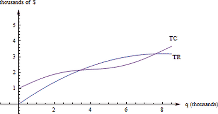
First, notice how to find the fixed cost and variable cost from the graph here. [latex]FC[/latex] is the [latex]y[/latex]-intercept of the [latex]TC[/latex] graph. ([latex]FC = TC(0)[/latex].) The graph of [latex]TVC[/latex] would have the same shape as the graph of [latex]TC[/latex], shifted down. ([latex]TVC = TC - FC[/latex].)
[latex]MC(q) = TC(x + 1) - TC(x)[/latex], but that’s impossible to read on this graph. How could you distinguish between [latex]TC(4022)[/latex] and [latex]TC(4023)[/latex]? On this graph, that interval is too small to see, and our best guess at the secant line is actually the tangent line to the [latex]TC[/latex] curve at that point. (This is the reason we want to have the derivative definition handy.)
[latex]MC(x)[/latex] is the slope of the tangent line to the [latex]TC[/latex] curve at [latex](x, TC(x))[/latex].
[latex]MR(x)[/latex] is the slope of the tangent line to the [latex]TR[/latex] curve at [latex](x, TR(x))[/latex].
Profit is the distance between the [latex]TR[/latex] and [latex]TC[/latex] curve. If you experiment with a clear ruler, you’ll see that the biggest profit occurs exactly when the tangent lines to the [latex]TR[/latex] and [latex]TC[/latex] curves are parallel. This is the rule that profit is maximized when [latex]MR = MC[/latex], or [latex]R'(x)=C'(x)[/latex] which we’ll explore later in the chapter.
Example 12
The demand, [latex]D[/latex], for a product at a price of [latex]p[/latex] dollars is given by [latex]D(p)=200-0.2p^2[/latex]. Find the marginal revenue when the price is $10.
Answer:
First we need to form a revenue equation. Since Revenue = Price[latex]\times[/latex]Quantity, and the demand equation shows the quantity of product that can be sold, we have \[R(p)=D(p)\cdot p=\left(200-0.2p^2\right)p=200p-0.2p^3\]
Now we can find marginal revenue by finding the derivative: \[R'(p)=200(1)-0.2(3p^2)=200-0.6p^2\]
At a price of $10, [latex]R'(10)=200-0.6(10)^2=140[/latex].
Notice the units for [latex]R'[/latex] are [latex]\frac{\text{dollars of Revenue}}{\text{dollar of price}}[/latex], so [latex]R'(10)=140[/latex] means that when the price is $10, the revenue will increase by $140 for each dollar that the price was increased.
Section Exercises
Work on the following exercises. Discuss your solutions with your peers and/or course instructor.
Section 2.3 Exercises – The Basic Rules for Derivatives
