7.2 Confidence Intervals for a Single Population Mean with Known Population Standard Deviation
LEARNING OBJECTIVES
- Calculate and interpret confidence intervals for estimating a population mean where the population standard deviation is known.
A confidence interval for a population mean with a known standard deviation is based on the fact that the sample means follow an approximately normal distribution. To construct a confidence interval for a single unknown population mean [latex]\mu[/latex], where the population standard deviation is known, we need [latex]\overline{x}[/latex], which is the point estimate of the unknown population mean [latex]\mu[/latex].
The confidence interval estimate will have the form:
[latex]\begin{eqnarray*}\text{Lower Limit}&=&\overline{x}-\text{margin of error}\\\\\text{Upper Limit}&=&\overline{x}-\text{margin of error}\end{eqnarray*}[/latex]
The margin of error depends on the confidence level. The confidence level is often considered the probability that the calculated confidence interval estimate will contain the true population parameter. However, it is more accurate to state that the confidence level is the percent of confidence intervals that contain the true population parameter when repeated samples are taken. Most often, it is the choice of the person constructing the confidence interval to choose a confidence level. Typically, confidence levels of [latex]90\%[/latex] or higher are used because we want to have a high level of certainty about the results.
Video: "Confidence Intervals - Introduction" by Joshua Emmanuel [3:35] is licensed under the Standard YouTube License.Transcript and closed captions available on YouTube.
EXAMPLE
Suppose we have collected data from a sample. The sample mean is [latex]7[/latex] and the margin of error is [latex]2.5[/latex].
The confidence interval is:
[latex]\begin{eqnarray*}\text{Lower Limit}&=&7-2.5=4.5\\\\\text{Upper Limit}&=&7+2.5=9.5\end{eqnarray*}[/latex]
If the confidence level is [latex]95\%[/latex], then we say that "We estimate with [latex]95\%[/latex] confidence that the true value of the population mean is between [latex]4.5[/latex] and [latex]9.5[/latex]."
TRY IT
Suppose we have data from a sample. The sample mean is [latex]15[/latex] and the margin of error is [latex]3.2[/latex]. What is the confidence interval estimate for the population mean?
Click to see Solution
[latex]\begin{eqnarray*}\text{Lower Limit}&=&15-3.2=11.8\\\\\text{Upper Limit}&=&15+3.2=18.2\end{eqnarray*}[/latex]
A confidence interval for a population mean with a known population standard deviation is based on the fact that the sample means follow an approximately normal distribution. Suppose that our sample has a mean of [latex]\overline{x}=10[/latex] and we have constructed the [latex]90\%[/latex] confidence interval with a lower limit of [latex]5[/latex] and an upper limit of [latex]15[/latex].
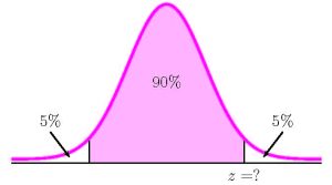
To get a [latex]90\%[/latex] confidence interval, we must include the central [latex]90\%[/latex] of the normal distribution. If we include the central [latex]90\%[/latex], we leave out a total of [latex]10\%[/latex] in both tails or [latex]5\%[/latex] in each tail of the normal distribution.
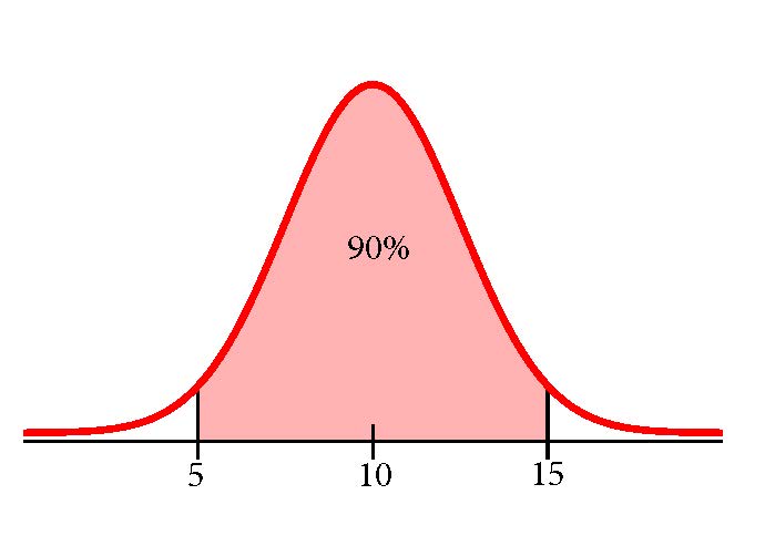
To capture the central [latex]90\%[/latex], we must go out [latex]1.645[/latex] "standard deviations" on either side of the calculated sample mean. The value [latex]1.645[/latex] is the [latex]z[/latex]-score from a standard normal distribution that puts an area of [latex]0.90[/latex] in the center, an area of [latex]0.05[/latex] in the far left tail, and an area of [latex]0.05[/latex] in the far right tail.
It is important that the "standard deviation" used is appropriate for the parameter we are estimating. So, in this section, we need to use the standard deviation that applies to sample means, which is [latex]\displaystyle{\frac{\sigma}{\sqrt{n}}}[/latex] (the standard deviation of the sample means). The fraction [latex]\displaystyle{\frac{\sigma}{\sqrt{n}}}[/latex] is commonly called the standard error of the mean in order to clearly distinguish the standard deviation for a sample mean from the population standard deviation [latex]\sigma[/latex].
Constructing the Confidence Interval
To construct a confidence interval estimate for an unknown population mean, we need data from a random sample. The steps to construct and interpret the confidence interval are:
- Calculate the sample mean [latex]\overline{x}[/latex] from the sample data. Remember, in this section, we already know the population standard deviation [latex]\sigma[/latex].
- Find the [latex]z[/latex]-score that corresponds to the confidence level [latex]C[/latex].
- Calculate the limits for the confidence interval.
- Write a sentence that interprets the estimate in the context of the problem. (Explain what the confidence interval means in the words of the problem.)
We will first examine each step in more detail and then illustrate the entire process with some examples.
Finding the [latex]z[/latex]-score for the Confidence Level
When we know the population standard deviation [latex]\sigma[/latex], we use a standard normal distribution to calculate the margin of error and construct the confidence interval. We need to find the value of [latex]z[/latex] that puts an area equal to the confidence level (in decimal form) in the middle of the standard normal distribution. The confidence level [latex]C[/latex] is the area in the middle of the standard normal distribution. The remaining area, [latex]1-C[/latex], is split equally between the two tails so that each of the tails contains an area equal to [latex]\displaystyle{\frac{1-C}{2}}[/latex].
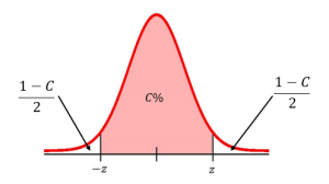
The [latex]z[/latex]-score needed to construct the confidence interval is the [latex]z[/latex]-score so that the entire area to the left of [latex]z[/latex]-score equals the area in the middle (the confidence level [latex]C[/latex]) plus the area in the left tail [latex]\displaystyle{\left(\frac{1-C}{2}\right)}[/latex]. That is, the required [latex]z[/latex]-score for the confidence interval is the [latex]z[/latex]-score so that the entire area to the left of the [latex]z[/latex]-score is
[latex]\displaystyle{C+\frac{1-C}{2}}[/latex]
For example, if the confidence level is [latex]95\%[/latex], then the area in the centre of the standard normal distribution is [latex]0.95[/latex] and the area in the left tail is [latex]\displaystyle{\frac{1-0.95}{2}=0.025}[/latex]. We would need to find the [latex]z[/latex]-score so that the entire area to the left of the [latex]z[/latex]-score equals [latex]0.95+0.025=0.975[/latex].
CALCULATING THE [latex]\color{white}{z}[/latex]-SCORE FOR A CONFIDENCE INTERVAL IN EXCEL
To find the [latex]z[/latex]-score to construct a confidence interval with confidence level [latex]C[/latex], use the norm.s.inv(area to the left of z) function.
- For area to the left of z, enter the entire area to the left of the [latex]z[/latex]-score required. For a confidence interval, the area to the left of [latex]z[/latex] is [latex]\displaystyle{C+\frac{1-C}{2}}[/latex].
The output from the norm.s.inv function is the value of [latex]z[/latex]-score needed to construct the confidence interval.
NOTE
The norm.s.inv function requires that we enter the entire area to the left of the unknown [latex]z[/latex]-score. This area includes the confidence level [latex]C[/latex] (the area in the middle of the distribution) plus the remaining area in the left tail [latex]\frac{1-C}{2}[/latex].
Calculating the Margin of Error
The margin of error for a confidence interval with confidence level [latex]C[/latex] for an unknown population mean [latex]\mu[/latex] when the population standard deviation [latex]\sigma[/latex] is known is
[latex]\displaystyle{\text{Margin of Error}=z\times\frac{\sigma}{\sqrt{n}}}[/latex]
where [latex]z[/latex] is the [latex]z[/latex]-score from the standard normal distribution so that the area to the left of [latex]z[/latex] is [latex]\displaystyle{C+\frac{1-C}{2}}[/latex].
Calculating the Limits of the Confidence Interval
The limits for the confidence interval with confidence level [latex]C[/latex] for an unknown population mean [latex]\mu[/latex] when the population standard deviation [latex]\sigma[/latex] is known are
[latex]\begin{eqnarray*}\text{Lower Limit}&=&\overline{x}-z\times\frac{\sigma}{\sqrt{n}}\\\\\text{Upper Limit}&=&\overline{x}+z\times\frac{\sigma}{\sqrt{n}}\end{eqnarray*}[/latex]
where [latex]z[/latex] is the [latex]z[/latex]-score from the standard normal distribution so that the area to the left of [latex]z[/latex] is [latex]\displaystyle{C+\frac{1-C}{2}}[/latex].

Interpreting a Confidence Interval
The interpretation should clearly state the confidence level [latex]C[/latex], explain what population parameter is being estimated (in this case, a population mean), and state the confidence interval (both endpoints). For example, "We estimate with ___% confidence that the true population mean (include the context of the problem) is between ___ and ___ (include appropriate units)."
Video: "Confidence Interval for a population mean - σ known" by Joshua Emmanuel [4:31] is licensed under the Standard YouTube License.Transcript and closed captions available on YouTube.
EXAMPLE
Suppose scores on exams in statistics are normally distributed with an unknown population mean and a population standard deviation of [latex]3[/latex] points. A random sample of [latex]36[/latex] scores is taken and has a sample mean of [latex]68[/latex] points.
- Find a [latex]90\%[/latex] confidence interval for the mean exam score.
- Interpret the confidence interval found in part 1.
- Is it reasonable to conclude that the mean exam score for all the exams is [latex]70[/latex]? Explain.
Solution
- To find the confidence interval, we need to find the [latex]z[/latex]-score for the [latex]90\%[/latex] confidence interval. This means that we need to find the [latex]z[/latex]-score from the standard normal distribution so that the entire area to the left of [latex]z[/latex] is [latex]\displaystyle{0.9+\frac{1-0.9}{2}=0.95}[/latex].
Function norm.s.inv Field 1 0.95 Answer 1.6448... So [latex]z=1.6448....[/latex]. From the question, [latex]\overline{x}=68[/latex], [latex]\sigma=3[/latex] and [latex]n=36[/latex]. The [latex]90\%[/latex] confidence interval is
[latex]\begin{eqnarray*}\\\text{Lower Limit}&=&\overline{x}-z\times\frac{\sigma}{\sqrt{n}}\\&=&68-1.6448...\times\frac{3}{\sqrt{36}}\\&=&67.18\\\\\text{Upper Limit}&=&\overline{x}+z\times\frac{\sigma}{\sqrt{n}}\\&=&68+1.6448...\times\frac{3}{\sqrt{36}}\\&=&68.82\\\\\end{eqnarray*}[/latex]
- We are [latex]90\%[/latex] confident that the mean exam score is between [latex]67.18[/latex] points and [latex]68.82[/latex] points.
- It is not reasonable to conclude that the mean exam score is [latex]70[/latex] points because [latex]70[/latex] points is outside the confidence interval. (In this case, there is a [latex]90\%[/latex] chance that the actual mean exam score is in between [latex]67.18[/latex] and [latex]68.82[/latex] and only a [latex]10\%[/latex] chance that the mean exam score is outside this interval. So it is unlikely (but not impossible) that the actual mean exam score is a value outside of the confidence interval.)
NOTES
- When calculating the limits for the confidence interval, keep all of the decimals in the [latex]z[/latex]-score and other values throughout the calculation. This will ensure that there is no round-off error in the answers. Use Excel to do the calculation of the limits, clicking on the cells containing the [latex]z[/latex]-score and any other values, to ensure that all of the decimal places are used in the calculation.
- When writing down the interpretation of the confidence interval, make sure to include the confidence level, the actual population mean captured by the confidence interval (i.e. be specific to the context of the question), and appropriate units for the limits.
- With a confidence level of [latex]C\%[/latex], [latex]C\%[/latex] of all confidence intervals constructed contain the true population parameter. For the above example, this means that [latex]90\%[/latex] of all confidence intervals constructed this way contain the true mean exam score. In other words, if we constructed [latex]100[/latex] of these confidence intervals (using [latex]100[/latex] different samples of size [latex]36[/latex]), we would expect [latex]90[/latex] of them to contain the true mean exam score.
TRY IT
Suppose average pizza delivery times are normally distributed with an unknown population mean and a population standard deviation of [latex]6[/latex] minutes. A random sample of [latex]28[/latex] pizza delivery restaurants is taken and has a sample mean delivery time of [latex]36[/latex] minutes.
- Find a [latex]96\%[/latex] confidence interval for the mean delivery time.
- Interpret the confidence interval found in part 1.
- Is it reasonable to claim that the mean delivery time is [latex]35[/latex] minutes? Explain.
Click to see Solution
-
Function norm.s.inv Field 1 0.98 Answer 2.053... 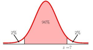 [latex]\begin{eqnarray*}\\\text{Lower Limit}&=&\overline{x}-z\times\frac{\sigma}{\sqrt{n}}\\&=&36-2.053...\times\frac{6}{\sqrt{28}}\\&=&33.67\\\\\text{Upper Limit}&=&\overline{x}+z\times\frac{\sigma}{\sqrt{n}}\\&=&36+2.053...\times\frac{6}{\sqrt{28}}\\&=&38.05\\\\\end{eqnarray*}[/latex]
 - We are [latex]96\%[/latex] confident that the mean delivery time is between [latex]33.67[/latex] minutes and [latex]38.05[/latex] minutes.
- It is reasonable to conclude that the mean delivery time is [latex]35[/latex] minutes because [latex]35[/latex] minutes is inside the confidence interval.

EXAMPLE
The Specific Absorption Rate (SAR) for a cell phone measures the amount of radio frequency (RF) energy absorbed by the user's body when using the handset. Every cell phone emits RF energy. Different phone models have different SAR measures. To receive certification from the Federal Communications Commission (FCC) for sale in the United States, the SAR level for a cell phone must be no more than [latex]1.6[/latex] watts per kilogram. This table shows the highest SAR level for a random selection of cell phone models as measured by the FCC.
| Phone Model | SAR | Phone Model | SAR | Phone Model | SAR |
|---|---|---|---|---|---|
| Apple iPhone 4S | 1.11 | LG Ally | 1.36 | Pantech Laser | 0.74 |
| BlackBerry Pearl 8120 | 1.48 | LG AX275 | 1.34 | Samsung Character | 0.5 |
| BlackBerry Tour 9630 | 1.43 | LG Cosmos | 1.18 | Samsung Epic 4G Touch | 0.4 |
| Cricket TXTM8 | 1.3 | LG CU515 | 1.3 | Samsung M240 | 0.867 |
| HP/Palm Centro | 1.09 | LG Trax CU575 | 1.26 | Samsung Messager III SCH-R750 | 0.68 |
| HTC One V | 0.455 | Motorola Q9h | 1.29 | Samsung Nexus S | 0.51 |
| HTC Touch Pro 2 | 1.41 | Motorola Razr2 V8 | 0.36 | Samsung SGH-A227 | 1.13 |
| Huawei M835 Ideos | 0.82 | Motorola Razr2 V9 | 0.52 | SGH-a107 GoPhone | 0.3 |
| Kyocera DuraPlus | 0.78 | Motorola V195s | 1.6 | Sony W350a | 1.48 |
| Kyocera K127 Marbl | 1.25 | Nokia 1680 | 1.39 | T-Mobile Concord | 1.38 |
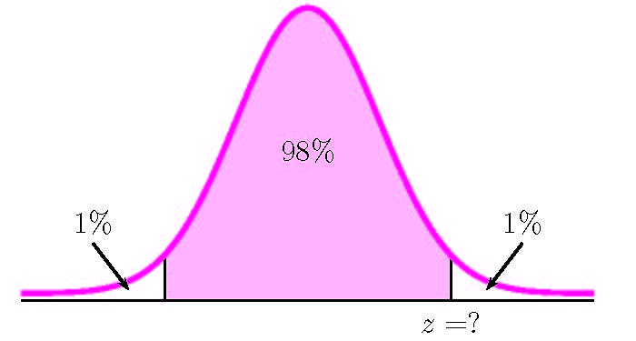
- Find a [latex]98\%[/latex] confidence interval for the mean of the Specific Absorption Rates (SARs) for cell phones. Assume that the population standard deviation is [latex]\sigma=0.337[/latex]
- Interpret the confidence interval found in part 1.
Solution
- To find the confidence interval, we need to find the [latex]z[/latex]-score for the [latex]98\%[/latex] confidence interval. This means that we need to find the [latex]z[/latex]-score from the standard normal distribution so that the entire area to the left of [latex]z[/latex] is [latex]\displaystyle{0.98+\frac{1-0.98}{2}=0.99}[/latex].

Function norm.s.inv Field 1 0.99 Answer 2.3263... So [latex]z=2.3263....[/latex]. From the sample data supplied in the question [latex]\overline{x}=1.0237...[/latex] and [latex]n=30[/latex]. The population standard deviation is [latex]\sigma=0.337[/latex]. The [latex]98\%[/latex] confidence interval is
[latex]\begin{eqnarray*}\\\text{Lower Limit}&=&\overline{x}-z\times\frac{\sigma}{\sqrt{n}}\\&=&1.0237...-2.3263...\times\frac{0.377}{\sqrt{30}}\\&=&0.8806\\\\\text{Upper Limit}&=&\overline{x}+z\times\frac{\sigma}{\sqrt{n}}\\&=&1.0237...+2.3262...\times\frac{0.377}{\sqrt{30}}\\&=&1.1839\\\\\end{eqnarray*}[/latex]
- We are [latex]98\%[/latex] confident that the mean of the Specific Absorption Rates is between [latex]0.8806[/latex] watts per kilogram and [latex]1.1839[/latex] watts per kilogram.
TRY IT
This table shows a different random sampling of [latex]20[/latex] cell phone models. Assume that the population standard deviation is [latex]\sigma=0.337[/latex].
| Phone Model | SAR | Phone Model | SAR |
|---|---|---|---|
| Blackberry Pearl 8120 | 1.48 | Nokia E71x | 1.53 |
| HTC Evo Design 4G | 0.8 | Nokia N75 | 0.68 |
| HTC Freestyle | 1.15 | Nokia N79 | 1.4 |
| LG Ally | 1.36 | Sagem Puma | 1.24 |
| LG Fathom | 0.77 | Samsung Fascinate | 0.57 |
| LG Optimus Vu | 0.462 | Samsung Infuse 4G | 0.2 |
| Motorola Cliq XT | 1.36 | Samsung Nexus S | 0.51 |
| Motorola Droid Pro | 1.39 | Samsung Replenish | 0.3 |
| Motorola Droid Razr M | 1.3 | Sony W518a Walkman | 0.73 |
| Nokia 7705 Twist | 0.7 | ZTE C79 | 0.869 |
- Construct a [latex]93\%[/latex] confidence interval for the mean SAR for cell phones certified for use in the United States.
- Interpret the confidence interval found in part 1.
Click to see Solution
-
Function norm.s.inv Field 1 0.965 Answer 1.8119... [latex]\begin{eqnarray*}\\\text{Lower Limit}&=&\overline{x}-z\times\frac{\sigma}{\sqrt{n}}\\&=&0.94...-1.8119...\times\frac{0.337}{\sqrt{20}}\\&=&0.8035\\\\\text{Upper Limit}&=&\overline{x}+z\times\frac{\sigma}{\sqrt{n}}\\&=&0.94...+1.8119...\times\frac{0.337}{\sqrt{20}}\\&=&1.0766\\\\\end{eqnarray*}[/latex]
- We are [latex]93\%[/latex] confident that the mean of the Specific Absorption Rates is between [latex]0.8035[/latex] watts per kilogram and [latex]1.0766[/latex] watts per kilogram.
NOTE
Notice the difference in the confidence intervals calculated in the Example and Try It just completed. These intervals are different for several reasons: they were calculated from different samples, the samples were different sizes, and the intervals were calculated for different levels of confidence. Even though the intervals are different, they do not yield conflicting information.
Changing the Confidence Level
EXAMPLE
Suppose scores on exams in statistics are normally distributed with an unknown population mean and a population standard deviation of [latex]3[/latex] points. A random sample of [latex]36[/latex] scores is taken and gives a sample mean of [latex]68[/latex] points. Previously, we found a [latex]90\%[/latex] confidence interval for the mean exam score. Now, find a [latex]95\%[/latex] confidence interval for the mean exam score. Interpret the [latex]95\%[/latex] confidence interval.
Solution
To find the confidence interval, we need to find the [latex]z[/latex]-score for the [latex]95\%[/latex] confidence interval. This means that we need to find the [latex]z[/latex]-score from the standard normal distribution so that the entire area to the left of [latex]z[/latex] is [latex]\displaystyle{0.95+\frac{1-0.95}{2}=0.975}[/latex].
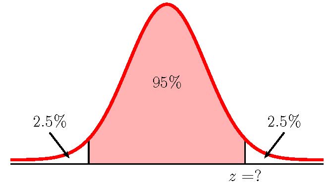
| Function | norm.s.inv |
|---|---|
| Field 1 | 0.975 |
| Answer | 1.9599... |
So [latex]z=1.9599....[/latex]. From the question [latex]\overline{x}=68[/latex], [latex]\sigma=3[/latex] and [latex]n=36[/latex]. The [latex]95\%[/latex] confidence interval is
[latex]\begin{eqnarray*}\\\text{Lower Limit}&=&\overline{x}-z\times\frac{\sigma}{\sqrt{n}}\\&=&68-1.9599...\times\frac{3}{\sqrt{36}}\\&=&67.02\\\\\text{Upper Limit}&=&\overline{x}+z\times\frac{\sigma}{\sqrt{n}}\\&=&68+1.9599...\times\frac{3}{\sqrt{36}}\\&=&68.98\\\\\end{eqnarray*}[/latex]
We are [latex]95\%[/latex] confident that the mean exam score is between [latex]67.02[/latex] points and [latex]68.98[/latex] points.
For the exam scores examples, the [latex]90\%[/latex] confidence interval has a lower limit of [latex]67.18[/latex] and an upper limit of [latex]68.82[/latex] and the [latex]95\%[/latex] confidence interval has a lower limit of [latex]67.02[/latex] and an upper limit of [latex]68.98[/latex]. Notice that the [latex]95\%[/latex] confidence interval is wider (the distance between the limits is larger in the [latex]95\%[/latex] confidence interval). If we look at the graphs, because the area [latex]0.95[/latex] is larger than the area [latex]0.90[/latex], it makes sense that the [latex]95\%[/latex] confidence interval is wider. To be more confident that the confidence interval actually contains the true value of the population mean for all statistics exam scores, the confidence interval necessarily needs to be wider.

When the confidence level increases, the margin of error increases, and the effect makes the confidence interval wider. When the confidence level decreases, the margin of error decreases, and the effect makes the confidence interval narrower.
Changing the Sample Size
EXAMPLE
Suppose scores on exams in statistics are normally distributed with an unknown population mean and a population standard deviation of [latex]3[/latex] points. Previously, we found a [latex]90\%[/latex] confidence interval for the mean exam score using a sample of size [latex]36[/latex] with a sample mean of [latex]68[/latex].
- Suppose everything is kept the same, but the sample size is [latex]100[/latex] (instead of [latex]36[/latex]). Find the [latex]90\%[/latex] confidence interval.
- Suppose everything is kept the same, but the sample size is [latex]25[/latex] (instead of [latex]36[/latex]). Find the [latex]90\%[/latex] confidence interval.
Solution
-
Function norm.s.inv Field 1 0.95 Answer 1.6448... [latex]\begin{eqnarray*}\\\text{Lower Limit}&=&\overline{x}-z\times\frac{\sigma}{\sqrt{n}}\\&=&68-1.6448...\times\frac{3}{\sqrt{100}}\\&=&67.51\\\\\text{Upper Limit}&=&\overline{x}+z\times\frac{\sigma}{\sqrt{n}}\\&=&68+1.6448...\times\frac{3}{\sqrt{100}}\\&=&68.49\\\\\end{eqnarray*}[/latex]
-
Function norm.s.inv Field 1 0.95 Answer 1.6448... [latex]\begin{eqnarray*}\\\text{Lower Limit}&=&\overline{x}-z\times\frac{\sigma}{\sqrt{n}}\\&=&68-1.6448...\times\frac{3}{\sqrt{25}}\\&=&67.01\\\\\text{Upper Limit}&=&\overline{x}+z\times\frac{\sigma}{\sqrt{n}}\\&=&68+1.6448...\times\frac{3}{\sqrt{25}}\\&=&69.27\end{eqnarray*}[/latex]
For the exam scores examples, the [latex]90\%[/latex] confidence interval with a sample size of [latex]36[/latex] has a lower limit of [latex]67.18[/latex] and an upper limit of [latex]68.82[/latex], with a sample size of [latex]100[/latex] has a lower limit of [latex]67.51[/latex] and an upper limit of [latex]68.49[/latex], and with a sample size of [latex]25[/latex] has a lower limit of [latex]67.01[/latex] and an upper limit of [latex]69.27[/latex]. When the sample size increases, the confidence interval is narrower. When the sample size decreases, the confidence interval is wider. Generally, the smaller the sample size, the wider the confidence interval needs to be in order to achieve the same level of confidence.
When the sample size increases, the margin of error decreases, and the effect makes the confidence interval narrower. When the sample size decreases, the margin of error increases, and the effect makes the confidence interval wider.
Exercises
- Statistics Canada conducts a study to determine the time needed to complete the short form of the census. Statistics Canada surveys [latex]200[/latex] people and found that the sample mean is [latex]8.2[/latex] minutes. The population standard deviation of [latex]2.2[/latex] minutes. The population distribution is assumed to be normal.
- Construct a [latex]90\%[/latex] confidence interval for the mean time to complete the short form of the census.
- Interpret the confidence interval found in part (a).
- Is it reasonable to conclude the mean time to complete the short form is [latex]10[/latex] minutes? Explain.
- If Statistics Canada wants to increase its level of confidence and keep the error bound the same by taking another survey, what changes should it make?
- If Statistics Canada did another survey, kept the error bound the same, and surveyed only [latex]50[/latex] people instead of [latex]200[/latex], what would happen to the level of confidence?
Click to see Answer
- [latex]\text{Lower Limit}=7.94[/latex], [latex]\text{Upper Limit}=8.46[/latex]
- There is a [latex]90\%[/latex] probability that the mean time to complete the short form of the census is between [latex]7.94[/latex] minutes and [latex]8.46[/latex] minutes.
- No, because [latex]10[/latex] minutes is outside the confidence interval.
- Increase the sample size.
- Confidence level would decrease.
- A sample of [latex]20[/latex] heads of lettuce was selected. The weight of each head of lettuce was then recorded. The mean weight from the sample was [latex]2.2[/latex] pounds. The population standard deviation is known to be [latex]0.2[/latex] pounds. Assume that the population distribution of head weight is normal.
- Construct a [latex]92\%[/latex] confidence interval for the population mean weight of the heads of lettuce.
- Interpret the confidence interval found in part (a).
- Construct a [latex]98\%[/latex] confidence interval for the population mean weight of the heads of lettuce.
- In complete sentences, explain why the confidence interval in part (c) is larger than in part (a).
- What would happen if [latex]40[/latex] heads of lettuce were sampled instead of [latex]20[/latex], and the error bound remained the same?
- What would happen if [latex]40[/latex] heads of lettuce were sampled instead of [latex]20[/latex], and the confidence level remained the same?
Click to see Answer
- [latex]\text{Lower Limit}=2.12[/latex], [latex]\text{Upper Limit}=2.28[/latex]
- There is a [latex]92\%[/latex] probability that the mean weight of heads of lettuce is between [latex]2.12[/latex] pounds and [latex]2.28[/latex] pounds.
- [latex]\text{Lower Limit}=2.10[/latex], [latex]\text{Upper Limit}=2.30[/latex]
- For the same sample size and sample data, a higher confidence level requires a wider interval to achieve the required accuracy.
- Confidence level would increase.
- The interval becomes narrower.
- A college wants to estimate the mean age of students entering the winter semester. Suppose that [latex]75[/latex] winter students were randomly selected, and the mean age for the sample was [latex]30.4[/latex] years. The population standard deviation of the ages of the students is [latex]15[/latex] years.
- Construct a [latex]99\%[/latex] confidence interval for the mean age of winter semester students at the college.
- Interpret the confidence interval found in part (a).
- Is it reasonable for the college to claim that the mean age of its winter semester students is [latex]35[/latex]? Explain.
- Using the same mean, standard deviation, and level of confidence, suppose that the sample size is [latex]69[/latex] instead of [latex]25[/latex]. Would the error bound become larger or smaller?
- Using the same mean, standard deviation, and sample size, how would the error bound change if the confidence level were reduced to [latex]90\%[/latex]?
Click to see Answer
- [latex]\text{Lower Limit}=25.94[/latex], [latex]\text{Upper Limit}=34.86[/latex]
- There is a [latex]99\%[/latex] probability that the mean age of winter semester students is between [latex]25.94[/latex] years and [latex]34.86[/latex] years.
- No, because [latex]35[/latex] is outside the confidence interval.
- Smaller.
- Error bound would get smaller.
- Suppose that an accounting firm does a study to determine the time needed to complete one person’s tax forms. It randomly surveys [latex]100[/latex] people and finds that the sample mean is [latex]23.6[/latex] hours. The population standard deviation of [latex]7.0[/latex] hours. The population distribution is assumed to be normal.
- Construct a [latex]97\%[/latex] confidence interval for the mean time to complete the tax forms.
- Interpret the confidence interval found in part (a).
- Is it reasonable for the firm to claim that the mean time to complete the tax forms is [latex]25[/latex] hours? Explain.
- If the firm wished to increase its level of confidence and keep the error bound the same by taking another survey, what changes should it make?
- If the firm did another survey, kept the error bound the same, and only surveyed [latex]49[/latex] people, what would happen to the level of confidence?
Click to see Answer
- [latex]\text{Lower Limit}=22.08[/latex], [latex]\text{Upper Limit}=25.12[/latex]
- There is a [latex]97\%[/latex] probability that the mean time to complete the tax forms is between [latex]22.08[/latex] hours and [latex]25.12[/latex] years.
- Yes, because [latex]25[/latex] is inside the confidence interval.
- Increase the sample size.
- Decreases.
- A sample of [latex]16[/latex] small bags of the same brand of candies was selected, and the mean weight was [latex]125[/latex] grams. Assume that the population distribution of bag weights is normal. The population standard deviation is known to be [latex]6.25[/latex] grams.
- Construct a [latex]90\%[/latex] confidence interval for the mean weight of the candies.
- Construct a [latex]98\%[/latex] confidence interval for the population mean weight of the candies.
- In complete sentences, explain why the confidence interval in part (b) is larger than the confidence interval in part (a).
- In complete sentences, give an interpretation of what the interval in part (b) means.
Click to see Answer
- [latex]\text{Lower Limit}=122.43[/latex], [latex]\text{Upper Limit}=127.57[/latex]
- [latex]\text{Lower Limit}=121.37[/latex], [latex]\text{Upper Limit}=128.63[/latex]
- For the same sample size and sample data, a higher confidence level requires a wider interval to achieve the required accuracy.
- There is a [latex]98\%[/latex] probability that the mean weight of the candies is between [latex]121.37[/latex] grams and [latex]128.63[/latex] years.
- What is meant by the term “[latex]90\%[/latex] confident” when constructing a confidence interval for a mean?
- If we took repeated samples, approximately [latex]90\%[/latex] of the samples would produce the same confidence interval.
- If we took repeated samples, approximately [latex]90\%[/latex] of the confidence intervals calculated from those samples would contain the sample mean.
- If we took repeated samples, approximately [latex]90\%[/latex] of the confidence intervals calculated from those samples would contain the true value of the population mean.
- If we took repeated samples, the sample mean would equal the population mean in approximately [latex]90\%[/latex] of the samples.
Click to see Answer
c
"7.2 Confidence Intervals for a Single Population Mean with Known Population Standard Deviation" and "7.6 Exercises" from Introduction to Statistics by Valerie Watts is licensed under a Creative Commons Attribution-NonCommercial-ShareAlike 4.0 International License, except where otherwise noted.
