5.1 Probability Distribution of a Continuous Random Variable
LEARNING OBJECTIONS
- Recognize and understand continuous probability distributions.
Previously, we learned about random variables. A continuous random variable corresponds to data that can be measured. Examples of continuous random variables include baseball batting averages, IQ scores, the length of time a long-distance telephone call lasts, the amount of money a person carries, the length of time a computer chip lasts, and SAT scores. Because the data is measured, there are an infinite number of numbers that a continuous random variable can take on, and so it is impossible to write down all of the numbers associated with a continuous random variable. Consequently, we represent the probability distribution of a continuous random variable with a graph and calculate probabilities associated with the continuous random variable by finding the corresponding area under the graph.
Continuous Probability Distributions
The graph of a probability distribution for a continuous random variable is a curve. The graph is defined so that the area between the curve and the [latex]x[/latex]-axis is equal to the probability. In other words, the probability a continuous random variable takes on a value in a specific interval is the area under the curve of the probability distribution of the continuous random variable.
Properties of a probability distribution for a continuous random variable include:
- The entire area under the curve of the distribution and above the [latex]x[/latex]-axis is equal to [latex]1[/latex].
- The probability that the continuous random variable takes on a value in between [latex]c[/latex] and [latex]d[/latex] is the area under the curve of the distribution in between [latex]x=c[/latex] and [latex]x=d[/latex].
- The probability that the continuous random variable exactly equals a particular number (i.e. the probability that the random variable takes on a specific number [latex]c[/latex]) is [latex]0[/latex]. (The area below the curve and above the [latex]x[/latex]-axis at the single point [latex]x=c[/latex] is a rectangle with height but no width. Therefore the area under the curve at [latex]x=c[/latex] is [latex]0[/latex], and so the probability is also [latex]0[/latex],
Generally, manual calculations to find the area under the curve of a continuous probability distribution is difficult, and most calculations require the use of computers. We will use the built-in functions in Excel to calculate the area under the continuous probability distribution functions. There are many different continuous probability distributions, including the uniform distribution and the exponential distribution. We will focus on the most important continuous probability distribution—the normal distribution.
NOTE
For a continuous random variable, the curve of the probability distribution is denoted by the function [latex]f(x)[/latex]. The function [latex]f(x)[/latex] is called a probability density function, and [latex]f(x)[/latex] produces the curve of the distribution. The function [latex]f(x)[/latex] is defined so that the area between it and the [latex]x[/latex]-axis is equal to a probability. The probability density function [latex]f(x)[/latex] itself does NOT give us probabilities associated with the continuous random variable. The function [latex]f(x)[/latex] produces the graph of the distribution, and the area under this graph corresponds to the probability.
EXAMPLE
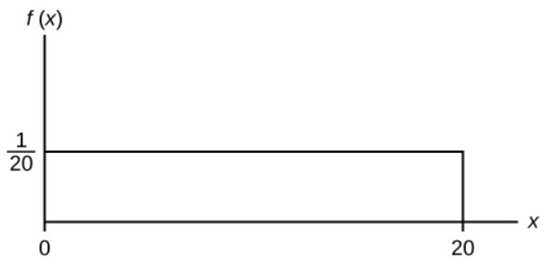
Suppose the graph below is the probability distribution of a continuous random variable. The graph is a horizontal line horizontal line segment from [latex]x=0[/latex] to [latex]x=20[/latex]. The height of the line is at [latex]\displaystyle\frac{1}{20}[/latex] for [latex]0\leq x\leq 20[/latex]. Note that the total area under the curve of [latex]f(x)[/latex], above the [latex]x[/latex]-axis, from [latex]x=0[/latex] to [latex]x=20[/latex] is
[latex]\displaystyle{\text{Area}=20\times\frac{1}{20}=1}[/latex]
Suppose we want to find the area between the curve and the [latex]x[/latex]-axis for [latex]0\lt x\lt 2[/latex].
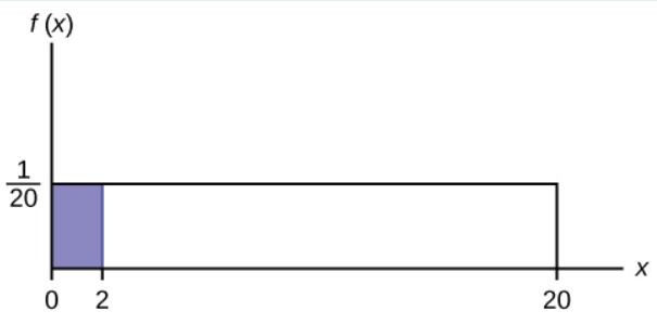
In this case, the area equals the area of a rectangle from [latex]x=0[/latex] to [latex]x=2[/latex]. The area of a rectangle is [latex]\text{base}\times\text{height}[/latex], so
[latex]\displaystyle{\text{Area}=(2-0)\times\frac{1}{20}=0.1}[/latex]
The area corresponds to the probability that the associated continuous random variable takes on a value between [latex]x=0[/latex] and [latex]x=2[/latex]. Because the area is [latex]0.1[/latex], the probability that [latex]0\lt x\lt 2[/latex] is [latex]0.1[/latex]. Mathematically, we can write this as:
[latex]\displaystyle{P(0\lt x\lt 2)=0.1}[/latex]
In other words, the probability that the random variable takes on a value between [latex]0[/latex] and [latex]2[/latex] is [latex]0.1[/latex].
Suppose we want to find the probability that the random variable takes on a value between [latex]x=4[/latex] and [latex]x=15[/latex]. This corresponds to the area under the curve in between [latex]x=4[/latex] and [latex]x=15[/latex].
[latex]\displaystyle{\text{Area}=(15-4)\times\frac{1}{20}=0.55}[/latex]
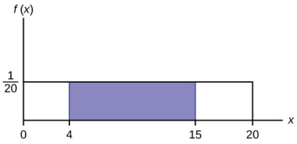
So, the probability that the random variable takes on a value between [latex]4[/latex] and [latex]15[/latex] is [latex]0.55[/latex].
Suppose we want to find [latex]P(x=15)[/latex]. This corresponds to the area above [latex]x=15[/latex], which is just a vertical line. A vertical line has no width (or zero width). So
[latex]\displaystyle{\text{Area}=0\times\frac{1}{20}=0}[/latex]
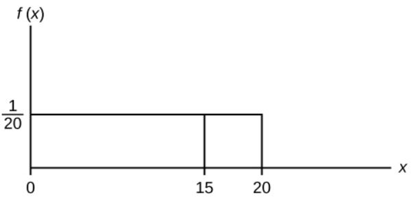
So, the probability that the random variable equals [latex]15[/latex] is [latex]0[/latex].
NOTE
The probability density function [latex]\displaystyle{f(x)=\frac{1}{20}}[/latex] used above is an example of a uniform distribution. The graph of a uniform distribution is always a horizontal line.
TRY IT
Suppose the graph shown below is a probability distribution for a continuous random variable. Find the probability that the random variable takes on a value between [latex]2.5[/latex] and [latex]7.5[/latex].
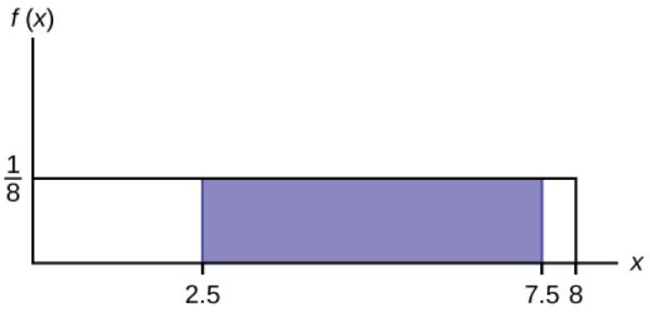
Click to see Solution
[latex]\displaystyle{\text{Area}=(7.5-2.5)\times\frac{1}{8}=0.625}[/latex]
Video: "Continuous probability distribution intro" by Khan Academy [9:58] is licensed under the Standard YouTube License.Transcript and closed captions available on YouTube.
"5.2 Probability Distribution of a Continuous Random Variable" and "5.6 Exercises" from Introduction to Statistics by Valerie Watts is licensed under a Creative Commons Attribution-NonCommercial-ShareAlike 4.0 International License, except where otherwise noted.
