11.2 Statistical Inference for Two Population Variances
LEARNING OBJECTIVES
- Construct and interpret a confidence interval for two population variances.
- Conduct and interpret a hypothesis test for two population variances.
Sometimes, we want to compare the variability between two populations, instead of comparing the means of the populations. For example, college administrators would like two college professors grading exams to have the same variation in their grading, or a supermarket might be interested in the variability of the check-out times for two checkers.
As with comparing other population parameters, we can construct confidence intervals and conduct hypothesis tests to study the relationship between two population variances. However, because of the distribution we need to use, we study the ratio of two population variances, not the difference in the variances.
Throughout this section, we will use subscripts to identify the values for the sample sizes, variances, and standard deviations for the two populations.
| Symbol for: | Population 1 | Population 2 |
|---|---|---|
| Population Variance | [latex]\sigma^2_1[/latex] | [latex]\sigma^2_2[/latex] |
| Population Standard Deviation | [latex]\sigma_1[/latex] | [latex]\sigma_2[/latex] |
| Sample Size | [latex]n_1[/latex] | [latex]n_2[/latex] |
| Sample Variance | [latex]s^2_1[/latex] | [latex]s^2_2[/latex] |
| Sample Standard Deviation | [latex]s_1[/latex] | [latex]s_2[/latex] |
In order to construct a confidence interval or conduct a hypothesis test on the ratio of two population variances, [latex]\displaystyle{\frac{\sigma_1^2}{\sigma^2_2}}[/latex], we need to use the distribution of [latex]\displaystyle{\frac{s_1^2}{s^2_2}}[/latex] when the population variances are equal ([latex]\sigma^2_1=\sigma^2_2[/latex]). Suppose we have two normal populations with equal variances [latex]\sigma^2_1=\sigma^2_2[/latex]. A sample of size [latex]n_1[/latex] with sample variance [latex]s^2_1[/latex] is taken from population [latex]1[/latex] and a sample of size [latex]n_2[/latex] with sample variance [latex]s^2_2[/latex] is taken from population [latex]2[/latex]. The sampling distribution of the ratio of the sample variances [latex]\displaystyle{\frac{s_1^2}{s_2^2}}[/latex] follows an [latex]F[/latex]-distribution with [latex]df_1=n_1-1[/latex] and [latex]df_2=n_2-1[/latex].
Constructing a Confidence Interval for the Ratio of Two Population Variances
Suppose a sample of size [latex]n_1[/latex] with sample variance [latex]s^2_1[/latex] is taken from population [latex]1[/latex] and a sample of size [latex]n_2[/latex] with sample variance [latex]s^2_2[/latex] is taken from population [latex]2[/latex], where the populations are independent and normally distributed. The limits for the confidence interval with confidence level [latex]C[/latex] for the ratio of the population variances [latex]\displaystyle{\frac{\sigma_1^2}{\sigma_2^2}}[/latex] are
[latex]\begin{eqnarray*}\\\text{Lower Limit}&=&\frac{1}{F_R}\times\frac{s_1^2}{s^2_2}\\\\\text{Upper Limit}&=&\frac{1}{F_L}\times\frac{s_1^2}{s^2_2}\\\\\end{eqnarray*}[/latex]
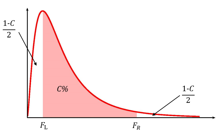
where [latex]F_L[/latex] is the [latex]F[/latex]-score so that the area in the left tail of the [latex]F[/latex]-distribution is [latex]\displaystyle{\frac{1-C}{2}}[/latex], [latex]F_R[/latex] is the [latex]F[/latex]-score so that the area in the right tail of the [latex]F[/latex]-distribution is [latex]\displaystyle{\frac{1-C}{2}}[/latex] and the [latex]F[/latex]-distribution has degrees of freedom [latex]df_1=n_1-1[/latex] and [latex]df_2=n_2-1[/latex].
NOTES
- Like the other confidence intervals we have seen, the [latex]F[/latex]-scores are the values that trap [latex]C\%[/latex] of the observations in the middle of the distribution so that the area of each tail is [latex]\displaystyle{\frac{1-C}{2}}[/latex].
- Because the [latex]F[/latex]-distribution is not symmetrical, the confidence interval for the ratio of the population variances requires that we calculate two different [latex]F[/latex]-scores: one for the left tail and one for the right tail. In Excel, we need to use both the f.inv function (for the left tail) and the f.inv.rt function (for the right tail) to find the two different [latex]F[/latex]-scores.
- The [latex]F[/latex]-score for the left tail is part of the formula for the upper limit, and the [latex]F[/latex]-score for the right tail is part of the formula for the lower limit. This is not a mistake. It follows from the formula used to determine the limits for the confidence interval.
- It is important that the populations are independent and normally distributed. If the populations are not normal, the confidence interval will not give an accurate result.
EXAMPLE
Two local walk-in medical clinics want to determine if there is any variability in the time patients wait to see a doctor at each clinic. In a sample of [latex]30[/latex] patients at Clinic 1, the standard deviation for the wait time to see a doctor was [latex]45[/latex] minutes. In a sample of 40 patients at Clinic 2, the standard deviation for the wait time to see a doctor was [latex]27[/latex] minutes. Assume the population of wait times at the two clinics are independent and normally distributed.
- Construct a [latex]95\%[/latex] confidence interval for the ratio of the variances for the wait times at the two clinics.
- Interpret the confidence interval found in part 1.
- Is there evidence to suggest that there is a difference in the variances of the wait times at the two clinics? Explain.
Solution
- Let Clinic 1 be population 1 and Clinic 2 be population 2. From the question, we have the following information:
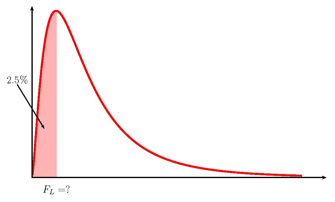
Clinic 1 Clinic 2 [latex]n_1=30[/latex] [latex]n_2=40[/latex] [latex]s_1^2=45^2=2025[/latex] [latex]s^2_2=27^2=729[/latex] To find the confidence interval, we need to find the [latex]F_L[/latex]-score for the [latex]95\%[/latex] confidence interval. This means that we need to find the [latex]F_L[/latex]-score so that the area in the left tail is [latex]\displaystyle{\frac{1-0.95}{2}=0.025}[/latex]. The degrees of freedom for the [latex]F[/latex]-distribution are [latex]df_1=n_1-1=30-1=29[/latex] and [latex]df_2=n_2-1=40-1=39[/latex].
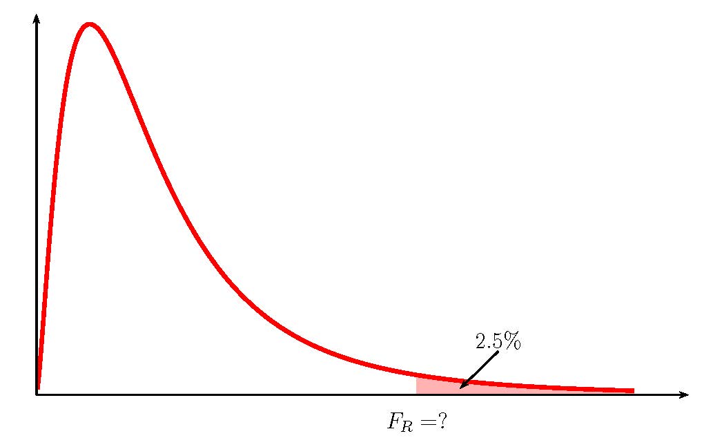
Function f.inv Field 1 0.025 Field 2 29 Field 3 39 Answer 0.4919... We also need to find the [latex]F_R[/latex]-score for the [latex]95\%[/latex] confidence interval. This means that we need to find the [latex]F_R[/latex]-score so that the area in the right tail is [latex]\displaystyle{\frac{1-0.95}{2}=0.025}[/latex]. The degrees of freedom for the [latex]F[/latex]-distribution are [latex]df_1=n_1-1=30-1=29[/latex] and [latex]df_2=n_2-1=40-1=39[/latex].

Function f.inv.rt Field 1 0.025 Field 2 29 Field 3 39 Answer 1.9618... So [latex]F_L=0.4919...[/latex] and [latex]F_R=1.9618...[/latex]. The [latex]95\%[/latex] confidence interval is
[latex]\begin{eqnarray*}\\\text{Lower Limit}&=&\frac{1}{F_R}\times\frac{s_1^2}{s^2_2}\\&=&\frac{1}{1.9618...}\times\frac{2025}{729}\\&=&1.416\\\\\text{Upper Limit}&=&\frac{1}{F_L}\times\frac{s_1^2}{s^2_2}\\&=&\frac{1}{0.4919...}\times\frac{2025}{729}\\&=&5.646\\\\\end{eqnarray*}[/latex]
- We are [latex]95\%[/latex] confident that the ratio of the variances in the wait times at the two clinics is between [latex]1.416[/latex] and [latex]5.646[/latex].
- Because [latex]1[/latex] is outside the confidence interval, it suggests that the ratio of the variances [latex]\displaystyle{\frac{\sigma^2_1}{\sigma^2_2}}[/latex] is not [latex]1[/latex]. If the ratio of the variances cannot equal [latex]1[/latex], then the variances cannot be equal. So there is a difference in the variances of the wait times at the two clinics.
NOTES
- When calculating the limits for the confidence interval, keep all of the decimals in the [latex]F[/latex]-scores and other values throughout the calculation. This will ensure that there is no round-off error in the answer. Use Excel to do the calculations of the limits, clicking on the cells containing the [latex]F[/latex]-scores and any other values.
- When writing down the interpretation of the confidence interval, make sure to include the confidence level and the actual ratio of population variances captured by the confidence interval (i.e. be specific to the context of the question).
TRY IT
A restauranteur knows that the mean revenue at her restaurant is higher on weekends than on weekdays. Now, she wants to investigate the variability in the revenue between weekends and weekdays. In a sample of [latex]13[/latex] weekday orders, the variance in the prices of the orders was [latex]63[/latex]. In a sample of [latex]11[/latex] weekend orders, the variance in the prices of the orders was [latex]181.25[/latex].
- Construct a [latex]99\%[/latex] confidence interval for the ratio of the variances in the prices between weekdays and weekends.
- Interpret the confidence interval found in part 1.
- Is there evidence to suggest that the variances in the prices is the same on weekdays and weekends? Explain.
Click to see Solution
Let weekday prices be population 1 and weekend prices be population 2.
-
Function f.inv Field 1 0.005 Field 2 12 Field 2 10 Answer 0.1966... Function f.inv.rt Field 1 0.005 Field 2 12 Field 3 10 Answer 5.661... [latex]\begin{eqnarray*}\text{Lower Limit}&=&\frac{1}{F_R}\times\frac{s_1^2}{s_2^2}\\&=&\frac{1}{5.661\ldots}\times\frac{63}{181.25}\\&=&0.0614\\\\\text{Upper Limit}&=&\frac{1}{F_L}\times\frac{s_1^2}{s_2^2}\\&=&\frac{1}{0.1966\ldots}\times\frac{63}{181.25}\\&=&1.7676\\\\\end{eqnarray*}[/latex]
- We are [latex]99\%[/latex] confident that the ratio of the variances in the prices on weekdays and weekends is between [latex]0.0614[/latex] and [latex]1.7676[/latex].
- Because [latex]1[/latex] is inside the confidence interval, it suggests that the ratio of the variances [latex]\displaystyle{\frac{\sigma^2_1}{\sigma^2_2}}[/latex] is equal to [latex]1[/latex]. If the ratio of the variances equals [latex]1[/latex], then the variances must be equal. So the variances in the prices on weekdays and weekends are the same.
Conducting a Hypothesis Test for Two Population Variances
Follow these steps to perform a hypothesis test on two population variances:
- Write down the null hypothesis that there is no difference in the population variances:
[latex]\begin{eqnarray*}\\H_0:&&\sigma^2_1=\sigma^2_2\end{eqnarray*}[/latex]
The null hypothesis is always the claim that the two population variances are equal.
- Write down the alternative hypotheses in terms of the difference in the population variances. The alternative hypothesis will be one of the following:
[latex]\begin{eqnarray*}\\H_a:&&\sigma^2_1\lt\sigma_2^2\\H_a:&&\sigma^2_1\gt\sigma^2_2\\H_a:&&\sigma^2_1\neq\sigma^2_2\\\\\end{eqnarray*}[/latex]
- Use the form of the alternative hypothesis to determine if the test is left-tailed, right-tailed, or two-tailed.
- Collect the sample information for the test and identify the significance level [latex]\alpha[/latex].
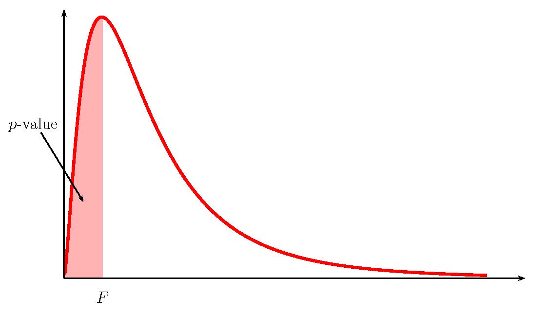
- Use the [latex]F[/latex]-distribution to find the [latex]p-\text{value}[/latex] (the area in the corresponding tail) for the test. The [latex]F[/latex]-score and degrees of freedom are
[latex]\begin{eqnarray*}F&=&\frac{s_1^2}{s_2^2}\\\\df_1&=&n_1-1\\\\df_2&=&n_2-1\\\\\end{eqnarray*}[/latex]
- Compare the [latex]p-\text{value}[/latex] to the significance level and state the outcome of the test.
- If [latex]p-\text{value}\leq\alpha[/latex], reject [latex]H_0[/latex] in favour of [latex]H_a[/latex].
- The results of the sample data are significant. There is sufficient evidence to conclude that the null hypothesis [latex]H_0[/latex] is an incorrect belief and that the alternative hypothesis [latex]H_a[/latex] is most likely correct.
- If [latex]p-\text{value}\gt\alpha[/latex], do not reject [latex]H_0[/latex].
- The results of the sample data are not significant. There is not sufficient evidence to conclude that the alternative hypothesis [latex]H_a[/latex] may be correct.
- If [latex]p-\text{value}\leq\alpha[/latex], reject [latex]H_0[/latex] in favour of [latex]H_a[/latex].
- Write down a concluding sentence specific to the context of the question.
EXAMPLE
Two college instructors are interested in whether or not there is any variation in the way they grade math exams. They each grade the same set of [latex]30[/latex] exams. The first instructor's grades have a variance of [latex]52.3[/latex]. The second instructor's grades have a variance of [latex]89.9[/latex]. At the [latex]5\%[/latex] significance level, test the claim that the first instructor's variance is smaller.
Solution
Let the first instructor's grades be population 1 and the second instructor's grades be population 2. From the question, we have the following information:
| Instructor 1 | Instructor 2 |
|---|---|
| [latex]n_1=30[/latex] | [latex]n_2=30[/latex] |
| [latex]s_1^2=52.3[/latex] | [latex]s_2^2=89.9[/latex] |
Hypotheses:
[latex]\begin{eqnarray*}H_0:&&\sigma_1^2=\sigma^2_2\\H_a:&&\sigma_1^2\lt\sigma^2_2\end{eqnarray*}[/latex]
[latex]p-\text{value}[/latex]:
Because the alternative hypothesis is a [latex]\lt[/latex], the [latex]p-\text{value}[/latex] is the area in the left tail of the [latex]F[/latex]-distribution.
To use the f.dist function, we need to calculate the [latex]F[/latex]-score and the degrees of freedom:
[latex]\begin{eqnarray*}F&=&\frac{s_1^2}{s_2^2}\\&=&\frac{52.3}{89.9}\\&=&0.58175...\\\\df_1&=&n_1-1\\&=&30-1\\&=&29\\\\df_2&=&n_2-1\\&=&30-1\\&=&29\end{eqnarray*}[/latex]
| Function | f.dist |
|---|---|
| Field 1 | 0.58175... |
| Field 2 | 29 |
| Field 3 | 29 |
| Field 4 | true |
| Answer | 0.0753 |
So the [latex]p-\text{value}=0.0753[/latex].
Conclusion:
Because [latex]p-\text{value}=0.0753\gt 0.05=\alpha[/latex], we do not reject the null hypothesis. At the [latex]5\%[/latex] significance level, there is not enough evidence to suggest that the first instructor's variance is smaller.
NOTES
- The null hypothesis [latex]\sigma_1^2=\sigma^2_2[/latex] is the claim that the variances for the two instructors are equal.
- The alternative hypothesis [latex]\sigma_1^2\lt\sigma^2_2[/latex] is the claim that the variance for the first instructor's grades is less than the variance for the second instructor's grades.
- The [latex]p-\text{value}[/latex] is the area in the left tail of the [latex]F[/latex]-distribution, to the left of [latex]F=0.5817...[/latex]. In the calculation of the [latex]p-\text{value}[/latex]:
- The function is f.dist because we are finding the area in the left tail of an [latex]F[/latex]-distribution.
- Field 1 is the value of [latex]F[/latex].
- Field 2 is the value of [latex]df_1[/latex].
- Field 3 is the value of [latex]df_2[/latex].
- Field 4 is true.
- The [latex]p-\text{value}[/latex] of [latex]0.0753[/latex] is a large probability compared to the significance level, and so is likely to happen assuming the null hypothesis is true. This suggests that the assumption that the null hypothesis is true is most likely correct, and so the conclusion of the test is to not reject the null hypothesis. In other words, the variances for the two instructors are most likely equal.
EXAMPLE
A local choral society divides the male singers into tenors and basses. The choral society director wants to know if the variance in the heights of the two groups of singers is the same or different. The director takes a sample from each group and records their height in inches. In a sample of [latex]22[/latex] tenors, the sample variance is [latex]3.89[/latex]. In a sample of [latex]27[/latex] basses, the sample variance is [latex]2.72[/latex]. At the [latex]5\%[/latex] significance level, is there a difference in the heights of the two groups of singers?
Solution
Let the tenors be population 1, and the basses be population 2. From the question, we have the following information:
| Tenors | Basses |
|---|---|
| [latex]n_1=22[/latex] | [latex]n_2=27[/latex] |
| [latex]s_1^2=3.89[/latex] | [latex]s^2=2.72[/latex] |
Hypotheses:
[latex]\begin{eqnarray*}H_0:&&\sigma^2_1=\sigma^2_2\\H_a:&&\sigma^2_1\neq\sigma^2_2\end{eqnarray*}[/latex]
[latex]p-\text{value}[/latex]:
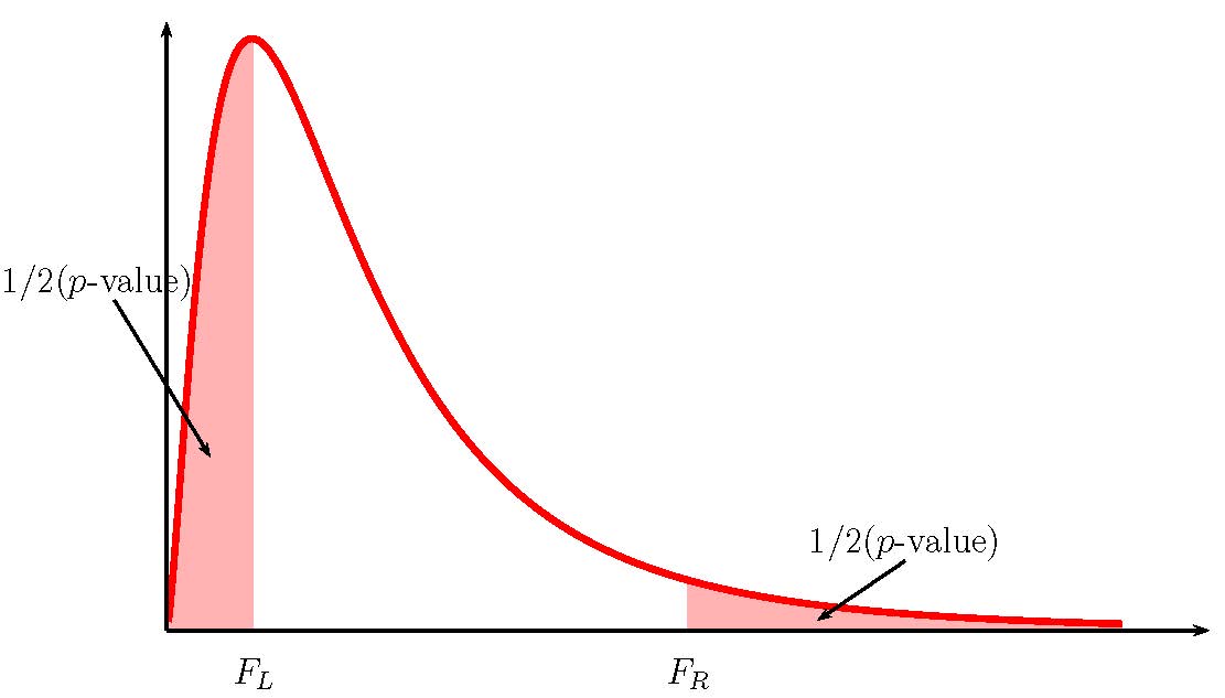
Because the alternative hypothesis is [latex]\neq[/latex], the [latex]p-\text{value}[/latex] is the sum of the areas in the tails of the [latex]F[/latex]-distribution.
We need to calculate out the [latex]F[/latex]-score and the degrees of freedom:
[latex]\begin{eqnarray*}F&=&\frac{s_1^2}{s_2^2}\\&=&\frac{3.89}{2.72}\\&=&1.430...\\\\df_1&=&n_1-1\\&=&22-1\\&=&21\\\\df_2&=&n_2-1\\&=&27-1\\&=&26\end{eqnarray*}[/latex]
Because this is a two-tailed test, we need to know which tail (left or right) we have the [latex]F[/latex]-score belongs to so that we can use the correct Excel function. If [latex]F\gt 1[/latex], the [latex]F[/latex]-score corresponds to the right tail. If the [latex]F\lt 1[/latex], the [latex]F[/latex]-score corresponds to the left tail. In this case, [latex]F=1.430...\gt 1[/latex], so the [latex]F[/latex]-score corresponds to the right tail. We need to use f.dist.rt to find the area in the right tail.
| Function | f.dist.rt |
|---|---|
| Field 1 | 1.430.... |
| Field 2 | 21 |
| Field 3 | 26 |
| Answer | 0.1919 |
So the area in the right tail is [latex]0.1919[/latex], which means that [latex]\frac{1}{2}p-\text{value}=0.1919[/latex]. This is also the area in the left tail, so
[latex]p-\text{value}=0.1919+0.1919=0.3838[/latex]
Conclusion:
Because [latex]p-\text{value}=0.3838\gt 0.05=\alpha[/latex], we do not reject the null hypothesis. At the [latex]5\%[/latex] significance level, there is not enough evidence to suggest that there is a difference in the variation in the heights of the two groups of singers.
NOTES
- The null hypothesis [latex]\sigma_1^2=\sigma^2_2[/latex] is the claim that the variances of the heights for the two groups of singers are equal.
- The alternative hypothesis [latex]\sigma_1^2\neq\sigma^2_2[/latex] is the claim that the variances of the heights for the two groups of singers are not equal
- In a two-tailed hypothesis test for two population variances, we will only have sample information relating to one of the two tails. We must determine which of the tails the sample information belongs to, and then calculate out the area in that tail. The area in each tail represents exactly half of the [latex]p-\text{value}[/latex], so the [latex]p-\text{value}[/latex] is the sum of the areas in the two tails.
- If [latex]F\lt 1[/latex], the sample information belongs to the left tail.
- We use f.dist to find the area in the left tail. The area in the right tail equals the area in the left tail, so we can find the [latex]p-\text{value}[/latex] by adding the output from this function to itself.
- If [latex]F\gt 1[/latex], the sample information belongs to the right tail.
- We use f.dist.rt to find the area in the right tail. The area in the left tail equals the area in the right tail, so we can find the [latex]p-\text{value}[/latex] by adding the output from this function to itself.
- If [latex]F\lt 1[/latex], the sample information belongs to the left tail.
- The [latex]p-\text{value}[/latex]of [latex]0.3838[/latex] is a large probability compared to the significance level, and so is likely to happen assuming the null hypothesis is true. This suggests that the assumption that the null hypothesis is true is most likely correct, and so the conclusion of the test is to not reject the null hypothesis In other words, the variances in the heights of the two groups of singers are the same.
NOTES
- When two populations have equal variances, the values of [latex]s_1^2[/latex] and [latex]s^2_2[/latex] are close in value. So, the value of [latex]\displaystyle{\frac{s^2_1}{s^2_2}}[/latex] is close to [latex]1[/latex]. This will result in a large [latex]p-\text{value}[/latex] in the hypothesis test, and the evidence favours the null hypothesis.
- When two populations have unequal variances, then the values of [latex]s_1^2[/latex] and [latex]s^2_2[/latex] are not close in value. So, the value of [latex]\displaystyle{\frac{s^2_1}{s^2_2}}[/latex] will either be larger than [latex]1[/latex] or smaller than [latex]1[/latex] (depending on which sample variance is smaller and which is larger). This will result in a small [latex]p-\text{value}[/latex] in the hypothesis test, and the evidence favours the alternative hypothesis.
TRY IT
A researcher knows that the mean annual repair costs for a car increases with the age of the car. But what about the variance in the repair costs? The researcher wants to know if the variance in the annual repair costs for cars increases as cars get older. In a sample of [latex]28[/latex] older (5 years or more) cars, the standard deviation of the annual repair costs was [latex]\$150[/latex]. In a sample of [latex]25[/latex] newer (3 years or less) cars, the standard deviation of the annual repair costs was [latex]\$90[/latex]. At the [latex]5\%[/latex] significance level, test if the variance in the annual repair costs is larger for older cars than for newer cars.
Click to see Solution
Let the older cars be population 1, and the newer cars be population 2.
Hypotheses:
[latex]\begin{eqnarray*}H_0:&&\sigma_1^2=\sigma_2^2\\H_a:&&\sigma_1^2\gt \sigma_2^2\end{eqnarray*}[/latex]
[latex]p-\text{value}[/latex]:
From the question, we have [latex]n_1=28[/latex], [latex]s_1^2=22,500[/latex], [latex]n_2=25[/latex], [latex]s_2^2=8,100[/latex], and [latex]\alpha=0.05[/latex].
Because the alternative hypothesis is a [latex]\gt[/latex], the [latex]p-\text{value}[/latex] is the area in the right tail of the [latex]F[/latex]-distribution.
To use the f.dist.rt function, we need to calculate out the [latex]\F[/latex]-score and the degrees of freedom:
[latex]\begin{eqnarray*}F&=&\frac{s_1^2}{s_2^2}\\&=&\frac{22,500}{8,100}\\&=&2.777\ldots\\\\df_1&=&n_1-1\\&=&28-1\\&=&27\\\\df_2&=&n_2-1\\&=&25-1\\&=&24\end{eqnarray*}[/latex]
| Function | f.dist.rt |
| Field 1 | 2.777... |
| Field 2 | 27 |
| Field 3 | 24 |
| Answer | 0.0068 |
So the [latex]p-\text{value}=0.0068[/latex].
Conclusion:
Because [latex]p-\text{value}=0.0068\lt 0.05=\alpha[/latex], we reject the null hypothesis. At the [latex]5\%[/latex] significance level there is enough evidence to suggest that the variance in the annual repair costs is larger for older cars than for newer cars.
Video: "Hypothesis Tests for Equality of Two Variances" by jbstatistics [11:40] is licensed under the Standard YouTube License.Transcript and closed captions available on YouTube.
Exercises
- As part of her capstone project, a business student is studying the starting salaries of accounting graduates and finance graduates. In a sample of [latex]35[/latex] accounting graduates, the starting salaries had a variance of [latex]137.2[/latex]. In a sample of [latex]30[/latex] finance graduates, the starting salaries had a variance of [latex]60.4[/latex].
- Construct a [latex]95\%[/latex] confidence interval for the ratio of the variances of the starting salaries of accounting and finance graduates.
- Interpret the confidence interval found in part (a).
- Is there evidence to suggest that the variance in the starting salaries of accounting graduates is higher than that of finance graduates? Explain.
Click to see Answer
- [latex]\text{Lower Limit}=1.101[/latex], [latex]\text{Upper Limit}=4.590[/latex]
- There is a [latex]95\%[/latex] probability that the ratio of the variances in the starting salaries of accounting and finance graduates is between [latex]1.101[/latex] and [latex]4.590[/latex].
- Yes. Because the lower limit is greater than [latex]1[/latex], it suggests that the ratio of the two variances is greater than [latex]1[/latex]. This can only happen if the variance for population 1 (accounting) is greater than the variance for population 2 (finance).
- Two co-workers commute from the same building. They are interested in whether or not there is any variation in the time it takes them to drive to work. They each record their times for [latex]20[/latex] commutes. The first worker’s times have a variance of [latex]12.1[/latex]. The second worker’s times have a variance of [latex]16.9[/latex]. At the [latex]5\%[/latex] significance level, test if the variation in the first worker's commute time is smaller than the second worker's.
Click to see Answer
- Hypotheses: [latex]\begin{eqnarray*}H_0:&&\sigma^2_1=\sigma^2_2\\H_a:&&\sigma^2_1\lt\sigma^2_2\end{eqnarray*}[/latex]
- [latex]p-\text{value}=0.2367[/latex]
- Conclusion: At the [latex]5\%[/latex] significance level, there is not enough evidence to conclude that the variation in the first worker's commute time is smaller than the variation in the second worker's.
- Two students are interested in whether or not there is variation in their test scores for math class. So far, they each have taken a total of [latex]15[/latex] total math tests. The first student’s grades have a standard deviation of [latex]38.1[/latex]. The second student’s grades have a standard deviation of [latex]22.5[/latex]. At the [latex]5\%[/latex] significance level, determine if the variation in the second student's scores are lower than the first student's.
Click to see Answer
- Hypotheses: [latex]\begin{eqnarray*}H_0:&&\sigma^2_1=\sigma^2_2\\H_a:&&\sigma^2_1\gt\sigma^2_2\end{eqnarray*}[/latex]
- [latex]p-\text{value}=0.0291[/latex]
- Conclusion: At the [latex]5\%[/latex] significance level, there is enough evidence to conclude that the variation in the second student's scores is lower than the variation in the first student's.
- Two cyclists are comparing the variances of their overall paces going uphill. In a sample of [latex]35[/latex] hill climbs, the first cyclist's speeds have a variance of [latex]23.8[/latex]. In a sample of [latex]40[/latex] hill climbs, the second cyclist's speeds have a variance of [latex]37.6[/latex]. At the [latex]5\%[/latex] significance level, is there a difference in the variance in the cyclists' speeds?
Click to see Answer
- Hypotheses: [latex]\begin{eqnarray*}H_0:&&\sigma^2_1=\sigma^2_2\\H_a:&&\sigma^2_1\neq\sigma^2_2\end{eqnarray*}[/latex]
- [latex]p-\text{value}=0.1775[/latex]
- Conclusion: At the [latex]5\%[/latex] significance level, there is not enough evidence to conclude that there is a difference in the variance in the cyclists' speeds.
- Students Linda and Tuan are given five laboratory rats each for a nutritional experiment. Each rat’s weight is recorded in grams. Linda feeds her rats Formula [latex]A[/latex], and Tuan feeds his rats Formula [latex]B[/latex]. At the end of a specified time period, each rat is weighed again, and the net gain in grams is recorded.
Linda's Rats Tuan's Rats 43.5 47.0 39.4 40.5 41.3 38.9 46.0 46.3 38.2 44.2 - Construct a [latex]98\%[/latex] confidence interval for the ratio of the variances in the net weight gain for Linda's and Tuan's rats.
- Interpret the confidence interval found in part (a).
- Is there evidence to suggest that the variance in the net weight gain for Linda and Tuan's rats is the same? Explain.
Click to see Answer
- [latex]\text{Lower Limit}=0.049[/latex], [latex]\text{Upper Limit}=12.433[/latex]
- There is a [latex]98\%[/latex] probability that the ratio of the variances in the net weight gain for Linda's and Tuan's rats is between [latex]0.049[/latex] and [latex]12.433[/latex].
- Yes. Because [latex]1[/latex] is inside the confidence interval, it suggests that the ratio of the two variances equals [latex]1[/latex]. If the ratio of the variances equals [latex]1[/latex], then the variances must be equal.
- A grassroots group opposed to a proposed increase in the gas tax claimed that the increase would hurt working-class people the most because they commute the farthest to work. Suppose that the group randomly surveyed [latex]16[/latex] individuals and asked them their daily one-way commuting distance, in kilometres. The results are shown in the table below.
Working-Class Professional (Middle Incomes) 17.8 16.5 26.7 17.4 49.4 22.0 9.4 7.4 65.4 9.4 47.1 2.1 19.5 6.4 51.2 13.9 Determine whether or not the variance in kilometres driven to work is statistically the same among the working class and professional (middle-income) groups. Use a [latex]5\%[/latex] significance level.
Click to see Answer
- Hypotheses: [latex]\begin{eqnarray*}H_0:&&\sigma^2_1=\sigma^2_2\\H_a:&&\sigma^2_1\neq\sigma^2_2\end{eqnarray*}[/latex]
- [latex]p-\text{value}=0.0096[/latex]
- Conclusion: At the [latex]5\%[/latex] significance level, there is enough evidence to conclude that there is a difference in the variance in the kilometres driven to work for the two groups.
- A researcher wants to study the variation in the amount of money, in dollars, that shoppers spend on Saturdays and Sundays at the mall. In a sample of [latex]12[/latex] Saturday shoppers, the standard deviation for the amount of money shoppers spent was [latex]\$43.2[/latex]. In a sample of [latex]16[/latex] Sunday shoppers, the standard deviation for the amount of money shoppers spent was [latex]\$38.3[/latex].
- Construct a [latex]93\%[/latex] confidence interval for the ratio of the variances for the amount of money spent by shoppers on Saturdays and Sundays at the mall.
- Interpret the confidence interval found in part (a).
- Is there evidence to suggest that variance in the amount of money spent on Saturdays and Sundays at the mall is different? Explain.
Click to see Answer
- [latex]\text{Lower Limit}=0.461[/latex], [latex]\text{Upper Limit}=3.848[/latex]
- There is a [latex]93\%[/latex] probability that the ratio of the variance in the amount of money spent by shoppers on Saturdays and Sundays at the mall is between [latex]0.461[/latex] and [latex]3.848[/latex].
- No. Because [latex]1[/latex] is inside the confidence interval, it suggests that the ratio of the two variances equals [latex]1[/latex]. If the ratio of the variances equals [latex]1[/latex], then the variances must be equal.
- A researcher is studying the incomes of people who live on the East Coast or West Coast. The table shows the results of the study. Income is shown in thousands of dollars. Assume that both distributions are normal.
East West 38 71 47 126 30 42 82 51 75 44 52 90 115 88 67 At the [latex]5\%[/latex] significance level, determine if the variation in income for people who live on the East Coast is lower than for people who live on the West Coast.
Click to see Answer
- Hypotheses: [latex]\begin{eqnarray*}H_0:&&\sigma^2_1=\sigma^2_2\\H_a:&&\sigma^2_1\lt\sigma^2_2\end{eqnarray*}[/latex]
- [latex]p-\text{value}=0.3912[/latex]
- Conclusion: At the [latex]5\%[/latex] significance level, there is not enough evidence to conclude that the variation in income for people who live on the East Coast is lower than for people who live on the West Coast.
- A financial planner is considering investing her client's money into one of two possible stock options, [latex]A[/latex] and [latex]B[/latex]. The client is risk adverse and wants to invest her money into a stock with the least amount of variability in the monthly percentage return of the stock. In a random sample of [latex]20[/latex] months of returns of stock [latex]A[/latex], the standard deviation is [latex]31.7\%[/latex]. In a random sample of [latex]30[/latex] months of returns of stock [latex]B[/latex], the standard deviation is [latex]19.5\%[/latex].
- At the [latex]1\%[/latex] significance level, is the variation in the monthly returns of stock [latex]A[/latex] greater than the variation in the monthly returns of stock [latex]B[/latex]?
- Which stock should the financial planner invest the client's money? Why?
Click to see Answer
-
- Hypotheses: [latex]\begin{eqnarray*}H_0:&&\sigma^2_1=\sigma^2_2\\H_a:&&\sigma^2_1\gt\sigma^2_2\end{eqnarray*}[/latex]
- [latex]p-\text{value}=0.0090[/latex]
- Conclusion: At the [latex]1\%[/latex] significance level, there is enough evidence to conclude that the variation in the monthly returns of stock [latex]A[/latex] is greater than the variation in the monthly returns of stock [latex]B[/latex].
- Stock [latex]B[/latex] because it has the smaller variation in the monthly returns.
- One of the measures of the quality of a production process is the variance in the process. A smaller variance means that there is more consistency in the product. A larger variance indicates that there is less consistency in the product. A company that produces [latex]500[/latex] gram bags of coffee uses two different machines in the bagging process. The company takes a sample of bags produced by each machine and records the weight, in grams, of each bag. The results are given in the table below.
Machine 1 Machine 2 495.5 501.3 502.7 499.9 495.9 500.7 498.6 498.2 501.6 500.4 502.5 498.7 499.2 499.2 496.7 496.3 498.7 498.1 499.0 500.1 499.3 499.8 498.8 499.3 499.1 500.2 500.8 500.1 499.3 497.5 497.2 499.6 498.1 499.6 499.4 497.7 499.2 499.6 498.2 498.8 497.7 499.7 498.8 500.3 At the [latex]1\%[/latex] significance level, is there a difference in the variance of the weights of the bags produced by each machine?
Click to see Answer
- Hypotheses: [latex]\begin{eqnarray*}H_0:&&\sigma^2_1=\sigma^2_2\\H_a:&&\sigma^2_1\neq\sigma^2_2\end{eqnarray*}[/latex]
- [latex]p-\text{value}=0.0652[/latex]
- Conclusion: At the [latex]1\%[/latex] significance level, there is not enough evidence to conclude that there is a difference in the variance of the weights of the bags produced by the two machines.
"11.3 Statistical Inference for Two Population Variances" and “11.5 Exercises” from Introduction to Statistics by Valerie Watts is licensed under a Creative Commons Attribution-NonCommercial-ShareAlike 4.0 International License, except where otherwise noted.
