10.4 The Test of Independence
LEARNING OBJECTIVES
- Conduct and interpret the [latex]\chi^2[/latex] test of independence.
Given two categorical variables, is there some relationship between the two categorical variables, or are the two categorical variables independent? The [latex]\chi^2[/latex] test of independence allows us to test if two categorical variables are independent (not related) or dependent (related). The test of independence can only show if a relationship exists between two variables, but the test does not show if one variable causes changes in the other variable.
The test of independence uses a contingency table to analyze the data. As we saw previously in probability, a contingency table lists the categories of one variable as the rows and the categories of the other variable as the columns. The frequency of a row-column combination is the number of items that occur in both categories.
Conducting a [latex]\chi^2[/latex] Test of Independence
Suppose one categorical variable has [latex]r[/latex] possible outcomes (categories) and the other categorical variable has [latex]c[/latex] possible outcomes (categories).
- Write down the null and alternative hypotheses:
[latex]\begin{eqnarray*}\\H_0:&&\text{The two categorical variables are independent}\\H_a:&&\text{The two categorical variables are dependent}\\\\\end{eqnarray*}[/latex]
- Collect the sample information for the test and identify the significance level [latex]\alpha[/latex].
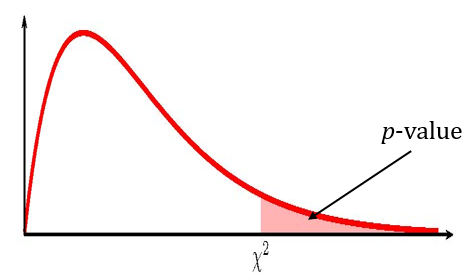
- Use the [latex]\chi^2[/latex]-distribution to find the [latex]p-\text{value}[/latex], which is the area in the right tail of the distribution. The [latex]\chi^2[/latex]-score and degrees of freedom are
[latex]\begin{eqnarray*}\chi^2&=&\sum\frac{(\text{observed-expected})^2}{\text{expected}}\\\\df&=&(r-1)\times(c-1)\\\\\text{observed}&=&\text{observed frequency from the sample data}\\\text{expected}&=&\frac{\text{row total}\times\text{column total}}{\text{table total}}\\r&=&\text{number of rows in the contingency table}\\c&=&\text{number of columns in the contingency table}\\\\\end{eqnarray*}[/latex]
- Compare the [latex]p-\text{value}[/latex] to the significance level and state the outcome of the test.
- If [latex]p-\text{value}\leq\alpha[/latex], reject [latex]H_0[/latex] in favour of [latex]H_a[/latex].
- The results of the sample data are significant. There is sufficient evidence to conclude that the null hypothesis [latex]H_0[/latex] is an incorrect belief and that the alternative hypothesis [latex]H_a[/latex] is most likely correct.
- If [latex]p-\text{value}\gt\alpha[/latex], do not reject [latex]H_0[/latex].
- The results of the sample data are not significant. There is not sufficient evidence to conclude that the alternative hypothesis [latex]H_a[/latex] may be correct.
- If [latex]p-\text{value}\leq\alpha[/latex], reject [latex]H_0[/latex] in favour of [latex]H_a[/latex].
- Write down a concluding sentence specific to the context of the question.
NOTES
- The null hypothesis is the claim that the two categorical variables are independent. That is, the null hypothesis claims that there is no relationship between the two categorical variables.
- The alternative hypothesis is the claim that the two categorical variables are dependent. That is, the alternative hypothesis claims that there is some relationship between the two categorical variables.
- The test can only show if a relationship exists between the two categorical variables. The test cannot show any type of causal relationship between the two categorical variables.
- The formula to find the expected frequencies follows from the assumption that the null hypothesis is true and how we calculate joint probabilities for independent events. Assuming the null hypothesis is true means that we assume the variables are independent. This means that we assume that the events in any row and column combination of the contingency tables are independent. As we saw in probability, when two events [latex]A[/latex] and [latex]B[/latex] are independent, [latex]P(A\text{ and }B)=P(A)\times P(B)[/latex]. Using this fact, we get the formula for the expected frequency: [latex]\displaystyle{\text{expected}=\frac{\text{row total}\times\text{column total}}{\text{table total}}}[/latex].
- In order to use the [latex]\chi^2[/latex] test of independence, the expected frequency for a cell in the contingency table must be at least [latex]5[/latex].
- The [latex]p-\text{value}[/latex] for a [latex]\chi^2[/latex] test of independence is always the area in the right tail of the [latex]\chi^2[/latex]-distribution. So, we use chisq.dist.rt to find the [latex]p-\text{value}[/latex] for a [latex]\chi^2[/latex] test of independence.
- To calculate the [latex]\chi^2[/latex]-score:
- For each of the possible outcomes of the categorical variables, calculate [latex]\displaystyle{\frac{(\text{observed-expected})^2}{\text{expected}}}[/latex]:
- Find the difference between the observed frequency (from the sample) and the expected frequency (from the null hypothesis). The expected frequency of any cell of the contingency table when the null hypothesis is true is: [latex]\displaystyle{\text{expected}=\frac{\text{row total}\times\text{column total}}{\text{table total}}}[/latex]
- Square the difference in step (i).
- Divide the value found in step (iii) by the expected frequency.
- Add up the values of [latex]\displaystyle{\frac{(\text{observed-expected})^2}{\text{expected}}}[/latex] for each of the outcomes.
- For each of the possible outcomes of the categorical variables, calculate [latex]\displaystyle{\frac{(\text{observed-expected})^2}{\text{expected}}}[/latex]:
EXAMPLE
A researcher is studying the relationship between drivers who commit speeding violations and drivers who use cell phones while driving. The researcher took a sample of [latex]755[/latex] drivers and obtained the information shown in the table below.
| Speeding violation in the last year | No speeding violation in the last year | Total | |
|---|---|---|---|
| Cell phone user | [latex]25[/latex] | [latex]280[/latex] | [latex]305[/latex] |
| Not a cell phone user | [latex]45[/latex] | [latex]405[/latex] | [latex]450[/latex] |
| Total | [latex]70[/latex] | [latex]685[/latex] | [latex]755[/latex] |
At the [latex]5\%[/latex] significance level, is there a relationship between drivers who commit speeding violations and drivers who use cell phones while driving?
Solution
Hypotheses:
[latex]\begin{eqnarray*}H_0:&&\text{The two variables are independent}\\H_a:&&\text{The two variables are dependent}\end{eqnarray*}[/latex]
[latex]p-\text{value}[/latex]:
From the question, we have [latex]r=2[/latex] and [latex]c=2[/latex]. Now we need to calculate out the [latex]\chi^2[/latex]-score for the test.
The observed frequency for each cell is the number of observations in the sample that fall into that cell. This is the information provided in the sample above.
| Observed Frequencies (Sample Data) |
|||
| Speeding violation in the last year | No speeding violation in the last year | Total | |
|---|---|---|---|
| Cell phone user | [latex]25[/latex] | [latex]280[/latex] | [latex]305[/latex] |
| Not a cell phone user | [latex]45[/latex] | [latex]405[/latex] | [latex]450[/latex] |
| Total | [latex]70[/latex] | [latex]685[/latex] | [latex]755[/latex] |
Next, we must calculate out the expected frequencies. Because we assume the null hypothesis is true (i.e. the variables are independent), the expected frequency in each cell is
[latex]\begin{eqnarray*}\text{expected}&=&\frac{\text{row total}\times\text{column total}}{\text{table total}}\end{eqnarray*}[/latex]
| Expected Frequencies |
|||
| Speeding violation in the last year | No speeding violation in the last year | Total | |
|---|---|---|---|
| Cell phone user | [latex]\displaystyle{\frac{305\times 70}{755}=28.27\ldots}[/latex] | [latex]\displaystyle{\frac{305\times 685}{755}=276.72\ldots}[/latex] | [latex]305[/latex] |
| Not a cell phone user | [latex]\displaystyle{\frac{450\times 70}{755}=41.72\ldots}[/latex] | [latex]\displaystyle{\frac{450\times 685}{755}=408.27\ldots}[/latex] | [latex]450[/latex] |
| Total | [latex]70[/latex] | [latex]685[/latex] | [latex]755[/latex] |
To calculate the [latex]\chi^2[/latex]-score for each cell, we work out the quantity [latex]\displaystyle{\frac{(\text{observed-expected})^2}{\text{expected}}}[/latex] and then add up these quantities.
[latex]\begin{eqnarray*}\chi^2&=&\sum\frac{(\text{observed-expected})^2}{\text{expected}}\\&=&\frac{(25-28.27\ldots)^2}{28.27\ldots}+\frac{(280-276.72\ldots)^2}{276.72\ldots}+\frac{(45-41.72\ldots)^2}{41.72\ldots}+\frac{(405-408.27\ldots)^2}{408.27\ldots}\\&=&0.7027\ldots\end{eqnarray*}[/latex]
The degrees of freedom for the [latex]\chi^2[/latex]-distribution is [latex]df=(r-1)\times(c-1)=(2-1)\times(2-1)=1[/latex]. The [latex]\chi^2[/latex] test of independence is a right-tailed test, so we use chisq.dist.rt function to find the [latex]p-\text{value}[/latex]:
| Function | chisq.dist.rt |
|---|---|
| Field 1 | 0.7027.... |
| Field 2 | 1 |
| Answer | 0.4019 |
So the [latex]p-\text{value}=0.4019[/latex].
Conclusion:
Because [latex]p-\text{value}=0.4019\gt 0.05=\alpha[/latex], we do not reject the null hypothesis. At the [latex]5\%[/latex] significance level, there is enough evidence to suggest that the two variables are independent.
NOTES
- The null hypothesis is the claim that the variables are independent. That is, there is no relationship between drivers who commit speeding violations and drivers who use cell phones while driving.
- The alternative hypothesis is the claim that the variables are dependent. That is, there is a relationship between drivers who commit speeding violations and drivers who use cell phones while driving.
- Keep all of the decimals throughout the calculation (i.e. in the calculation of the [latex]\chi^2[/latex]-score) to avoid any round-off error in the calculation of the [latex]p-\text{value}[/latex]. This ensures that we get the most accurate value for the [latex]p-\text{value}[/latex].
- The [latex]p-\text{value}[/latex] is the area in the right tail of the [latex]\chi^2[/latex]-distribution, to the right of [latex]\chi^2=0.7027...[/latex]. In the calculation of the [latex]p-\text{value}[/latex]:
- The function is chisq.dist.rt because we are finding the area in the right tail of a [latex]\chi^2[/latex]-distribution.
- Field 1 is the value of [latex]\chi^2[/latex].
- Field 2 is the value of the degrees of freedom [latex]df[/latex].
- The [latex]p-\text{value}[/latex] of [latex]0.4019[/latex] is a large probability compared to the significance level, and so is likely to happen assuming the null hypothesis is true. This suggests that the assumption that the null hypothesis is true is most likely correct, and so the conclusion of the test is to not reject the null hypothesis. In other words, the two variables are independent.
EXAMPLE
In a volunteer group, adults 21 and older volunteer from one to nine hours each week to spend time with a disabled senior citizen. The program recruits among college students, university students, and non-students. The table below is a sample of the adult volunteers and the number of hours they volunteer per week.
| 1-3 Hours | 4-6 Hours | 7-9 Hours | Total | |
|---|---|---|---|---|
| College Students | [latex]111[/latex] | [latex]96[/latex] | [latex]48[/latex] | [latex]255[/latex] |
| University Students | [latex]96[/latex] | [latex]133[/latex] | [latex]61[/latex] | [latex]290[/latex] |
| Non Students | [latex]91[/latex] | [latex]150[/latex] | [latex]53[/latex] | [latex]294[/latex] |
| Total | [latex]298[/latex] | [latex]379[/latex] | [latex]162[/latex] | [latex]839[/latex] |
At the [latex]5\%[/latex] significance level, is the number of hours volunteered independent of the type of volunteer?
Solution
Hypotheses:
[latex]\begin{eqnarray*}H_0:&&\text{The two variables are independent}\\H_a:&&\text{The two variables are dependent}\end{eqnarray*}[/latex]
[latex]p-\text{value}[/latex]:
From the question, we have [latex]r=3[/latex] and [latex]c=3[/latex]. Now we need to calculate out the [latex]\chi^2[/latex]-score for the test.
The observed frequency for each cell is the number of observations in the sample that fall into that cell. This is the information provided in the sample above.
| Observed Frequencies (Sample Data) |
||||
| 1-3 Hours | 4-6 Hours | 7-9 Hours | Total | |
|---|---|---|---|---|
| College Students | [latex]111[/latex] | [latex]96[/latex] | [latex]48[/latex] | [latex]255[/latex] |
| University Students | [latex]96[/latex] | [latex]133[/latex] | [latex]61[/latex] | [latex]290[/latex] |
| Non Students | [latex]91[/latex] | [latex]150[/latex] | [latex]53[/latex] | [latex]294[/latex] |
| Total | [latex]298[/latex] | [latex]379[/latex] | [latex]162[/latex] | [latex]839[/latex] |
Next, we must calculate out the expected frequencies. Because we assume the null hypothesis is true (i.e. the variables are independent), the expected frequency in each cell is
[latex]\begin{eqnarray*}\text{expected}&=&\frac{\text{row total}\times\text{column total}}{\text{table total}}\end{eqnarray*}[/latex]
| Expected Frequencies |
||||
| 1-3 Hours | 4-6 Hours | 7-9 Hours | Total | |
|---|---|---|---|---|
| College Students | [latex]\displaystyle{\frac{255\times 298}{839}=90.57\ldots}[/latex] | [latex]\displaystyle{\frac{255\times 379}{839}=115.19\ldots}[/latex] | [latex]\displaystyle{\frac{255\times 162}{839}=49.23\ldots}[/latex] | [latex]255[/latex] |
| University Students | [latex]\displaystyle{\frac{290\times 298}{839}=103.00\ldots}[/latex] | [latex]\displaystyle{\frac{290\times 379}{839}=131.00\ldots}[/latex] | [latex]\displaystyle{\frac{290\times 162}{839}=55.99\ldots}[/latex] | [latex]290[/latex] |
| Non Students | [latex]\displaystyle{\frac{294\times 298}{839}=104.42\ldots}[/latex] | [latex]\displaystyle{\frac{294\times 379}{839}=132.80\ldots}[/latex] | [latex]\displaystyle{\frac{294\times 162}{839}=56.76\ldots}[/latex] | [latex]294[/latex] |
| Total | [latex]298[/latex] | [latex]379[/latex] | [latex]162[/latex] | [latex]839[/latex] |
To calculate the [latex]\chi^2[/latex]-score for each cell, we work out the quantity [latex]\displaystyle{\frac{(\text{observed-expected})^2}{\text{expected}}}[/latex] and then add up these quantities.
[latex]\begin{eqnarray*}\chi^2&=&\sum\frac{(\text{observed-expected})^2}{\text{expected}}\\&=&\frac{(111-90.57\ldots)^2}{90.57\ldots}+\frac{(96-115.19\ldots)^2}{115.19\ldots}+\frac{(48-49.23\ldots)^2}{49.23\ldots}\\&&+\frac{(96-103.00\ldots)^2}{103.00\ldots}+\frac{(133-131.00\ldots)^2}{131.00\ldots}+\frac{(61-55.99\ldots)^2}{55.99\ldots}\\&&+\frac{(91-104.42\ldots)^2}{104.42\ldots}+\frac{(150-132.80\ldots)^2}{132.80\ldots}+\frac{(53-56.76\ldots)^2}{56.76\ldots}\\&=&12.99\ldots\end{eqnarray*}[/latex]
The degrees of freedom for the [latex]\chi^2[/latex]-distribution is [latex]df=(r-1)\times(c-1)=(3-1)\times(3-1)=4[/latex]. The [latex]\chi^2[/latex] test of independence is a right-tailed test, so we use chisq.dist.rt function to find the [latex]p-\text{value}[/latex]:
| Function | chisq.dist.rt |
|---|---|
| Field 1 | 12.99.... |
| Field 2 | 4 |
| Answer | 0.0113 |
So the [latex]p-\text{value}=0.0113[/latex].
Conclusion:
Because [latex]p-\text{value}=0.0113\lt 0.05=\alpha[/latex], we reject the null hypothesis in favour of the alternative hypothesis. At the [latex]5\%[/latex] significance level, there is enough evidence to suggest that the number of hours volunteered and the type of volunteer are dependent.
NOTES
- The null hypothesis is the claim that the variables are independent. That is, there is no relationship between the number of hours volunteered and the type of volunteer.
- The alternative hypothesis is the claim that the variables are dependent. That is, there is a relationship between the number of hours volunteered and the type of volunteer.
- Keep all of the decimals throughout the calculation (i.e. in the calculation of the [latex]\chi^2[/latex]-score) to avoid any round-off error in the calculation of the [latex]p-\text{value}[/latex]. This ensures that we get the most accurate value for the [latex]p-\text{value}[/latex].
- The [latex]p-\text{value}[/latex] of [latex]0.0113[/latex] is a small probability compared to the significance level, and so is unlikely to happen assuming the null hypothesis is true. This suggests that the assumption that the null hypothesis is true is most likely incorrect, and so the conclusion of the test is to reject the null hypothesis in favour of the alternative hypothesis. In other words, the two variables are dependent.
TRY IT
In a local school district, a music teacher wants to study the relationship between students who take music and students on the honour roll. The teacher took a sample of [latex]300[/latex] students and obtained the information shown in the table below.
| Honour Roll Student | Non-Honour Roll Student | Total | |
|---|---|---|---|
| Music Student | [latex]24[/latex] | [latex]26[/latex] | [latex]50[/latex] |
| Non-Music Student | [latex]67[/latex] | [latex]183[/latex] | [latex]250[/latex] |
| Total | [latex]97[/latex] | [latex]203[/latex] | [latex]300[/latex] |
At the [latex]5\%[/latex] significance level, is there a relationship between music/non-music students and honour roll/non-honour roll students?
Click to see Solution
Hypotheses:
[latex]\begin{eqnarray*}H_0:&&\text{The two variables are independent}\\H_a:&&\text{The two variables are dependent}\end{eqnarray*}[/latex]
[latex]p-\text{value}[/latex]:
From the question, we have [latex]r=2[/latex] and [latex]c=2[/latex].
| Observed Frequencies (Sample Data) |
|||
| Honour Roll Student | Non-Honour Roll Student | Total | |
|---|---|---|---|
| Music Student | [latex]24[/latex] | [latex]26[/latex] | [latex]50[/latex] |
| Non-Music Student | [latex]67[/latex] | [latex]183[/latex] | [latex]250[/latex] |
| Total | [latex]97[/latex] | [latex]203[/latex] | [latex]300[/latex] |
| Expected Frequencies |
|||
| Honour Roll Student | Non-Honour Roll Student | Total | |
|---|---|---|---|
| Music Student | [latex]16.166\ldots[/latex] | [latex]33.833\ldots[/latex] | [latex]50[/latex] |
| Non-Music Student | [latex]80.833\ldots[/latex] | [latex]169.166\ldots[/latex] | [latex]250[/latex] |
| Total | [latex]97[/latex] | [latex]203[/latex] | [latex]300[/latex] |
[latex]\begin{eqnarray*}\chi^2&=&\sum\frac{(\text{observed-expected})^2}{\text{expected}}\\&=&\frac{(24-16.166\ldots)^2}{16.166\ldots}+\frac{(26-33.833\ldots)^2}{33.833\ldots}+\frac{(67-80.833\ldots)^2}{80.833\ldots}+\frac{(183-169.166\ldots)^2}{169.165\ldots.}\\&=&9.107\ldots\\\\df&=&(r-1)\times(c-1)\\&=&(2-1)\times(2-1)\\&=&1\end{eqnarray*}[/latex]
| Function | chisq.dist.rt |
|---|---|
| Field 1 | 9.107... |
| Field 2 | 1 |
| Answer | 0.0025 |
So the [latex]p-\text{value}=0.0025[/latex].
Conclusion:
Because [latex]p-\text{value}=0.0025\lt 0.05=\alpha[/latex], we reject the null hypothesis in favour of the alternative hypothesis. At the [latex]5\%[/latex] significance level, there is enough evidence to suggest that the two variables are dependent.
TRY IT
A local college is interested in the relationship between student anxiety level and the need to succeed in school. A random sample of [latex]400[/latex] students took a test that measured anxiety level and the need to succeed in school. The results are shown in the table below.
| High Anxiety | Med-High Anxiety | Medium Anxiety | Med-Low Anxiety | Low Anxiety | Total | |
|---|---|---|---|---|---|---|
| High Need | [latex]35[/latex] | [latex]42[/latex] | [latex]53[/latex] | [latex]15[/latex] | [latex]10[/latex] | [latex]155[/latex] |
| Medium Need | [latex]18[/latex] | [latex]48[/latex] | [latex]63[/latex] | [latex]33[/latex] | [latex]31[/latex] | [latex]193[/latex] |
| Low Need | [latex]4[/latex] | [latex]5[/latex] | [latex]11[/latex] | [latex]15[/latex] | [latex]17[/latex] | [latex]52[/latex] |
| Total | [latex]57[/latex] | [latex]95[/latex] | [latex]127[/latex] | [latex]63[/latex] | [latex]58[/latex] | [latex]400[/latex] |
At the [latex]5\%[/latex] significance level, is there a relationship between student anxiety level and the need to succeed in school?
Click to see Solution
Hypotheses:
[latex]\begin{eqnarray*}H_0:&&\text{The two variables are independent}\\H_a:&&\text{The two variables are dependent}\end{eqnarray*}[/latex]
[latex]p-\text{value}[/latex]:
From the question, we have [latex]r=3[/latex] and [latex]c=5[/latex].
| Observed Frequencies (Sample Data) |
||||||
| High Anxiety | Med-High Anxiety | Medium Anxiety | Med-Low Anxiety | Low Anxiety | Total | |
|---|---|---|---|---|---|---|
| High Need | [latex]35[/latex] | [latex]42[/latex] | [latex]53[/latex] | [latex]15[/latex] | [latex]10[/latex] | [latex]155[/latex] |
| Medium Need | [latex]18[/latex] | [latex]48[/latex] | [latex]63[/latex] | [latex]33[/latex] | [latex]31[/latex] | [latex]193[/latex] |
| Low Need | [latex]4[/latex] | [latex]5[/latex] | [latex]11[/latex] | [latex]15[/latex] | [latex]17[/latex] | [latex]52[/latex] |
| Total | [latex]57[/latex] | [latex]95[/latex] | [latex]127[/latex] | [latex]63[/latex] | [latex]58[/latex] | [latex]400[/latex] |
| Expected Frequencies |
||||||
| High Anxiety | Med-High Anxiety | Medium Anxiety | Med-Low Anxiety | Low Anxiety | Total | |
|---|---|---|---|---|---|---|
| High Need | [latex]22.08\ldots[/latex] | [latex]36.81\ldots[/latex] | [latex]49.21\ldots[/latex] | [latex]24.41\ldots[/latex] | [latex]22.47\ldots[/latex] | [latex]155[/latex] |
| Medium Need | [latex]27.50\ldots[/latex] | [latex]45.83\ldots[/latex] | [latex]61.27\ldots[/latex] | [latex]30.39\ldots[/latex] | [latex]27.98\ldots[/latex] | [latex]193[/latex] |
| Low Need | [latex]7.41[/latex] | [latex]12.35[/latex] | [latex]16.51[/latex] | [latex]8.19[/latex] | [latex]7.54[/latex] | [latex]52[/latex] |
| Total | [latex]57[/latex] | [latex]95[/latex] | [latex]127[/latex] | [latex]63[/latex] | [latex]58[/latex] | [latex]400[/latex] |
[latex]\begin{eqnarray*}\chi^2&=&\sum\frac{(\text{observed-expected})^2}{\text{expected}}\\&=&\frac{(35-22.08\ldots)^2}{22.08\ldots}+\frac{(18-27.50\ldots)^2}{27.50\ldots}+\frac{(4-7.41)^2}{7.41}\\&&+\frac{(42-36.81\ldots)^2}{36.81\ldots}+\frac{(48-45.83\ldots)^2}{45.83\ldots}+\frac{(5-12.35)^2}{12.35}\\&&+\frac{(53-49.21\ldots)^2}{49.21\ldots}+\frac{(63-61.27\ldots)^2}{61.27\ldots}+\frac{(11-16.51)^2}{16.51}\\&&+\frac{(15-24.41\ldots)^2}{24.41\ldots}+\frac{(33-30.39\ldots)^2}{30.39\ldots}+\frac{(15-8.19)^2}{8.19}\\&&+\frac{(10-22.47\ldots)^2}{22.47\ldots}+\frac{(31-27.98\ldots)^2}{27.98\ldots}+\frac{(17-7.54)^2}{7.54}\\&=&48.419\ldots\\\\df&=&(r-1)\times(c-1)\\&=&(3-1)\times(5-1)\\&=&8\end{eqnarray*}[/latex]
| Function | chisq.dist.rt |
|---|---|
| Field 1 | 48.419... |
| Field 2 | 8 |
| Answer | 0.00000008 |
So the [latex]p-\text{value}=0.00000008[/latex].
Conclusion:
Because [latex]p-\text{value}=0.00000008\lt 0.05=\alpha[/latex], we reject the null hypothesis in favour of the alternative hypothesis. At the [latex]5\%[/latex] significance level, there is enough evidence to suggest that the two variables are dependent.
Video: "Chi-square test for association (independence) | AP Statistics | Khan Academy" by Khan Academy [10:28] is licensed under the Standard YouTube License.Transcript and closed captions available on YouTube.
Exercises
- Transit Railroads is interested in the relationship between travel distance and the ticket class purchased. A random sample of [latex]200[/latex] passengers is taken. The table below shows the results. At the [latex]5\%[/latex] significance level, determine if a passenger’s choice in ticket class is independent of the distance they must travel.
Travelling Distance Third class Second class First class Total 1–100 km 21 14 6 41 101–200 km 18 16 8 42 201–300 km 16 17 15 48 301–400 km 12 14 21 47 401–500 km 6 6 10 22 Total 73 67 60 200 Click to see Answer
- Hypotheses: [latex]\begin{eqnarray*}H_0:&&\text{The two variables are independent}\\H_a:&&\text{The two variables are dependent}\end{eqnarray*}[/latex]
- [latex]p-\text{value}=0.0435[/latex]
- Conclusion: At the [latex]5\%[/latex] significance level, there is enough evidence to conclude that a passenger's choice of ticket and distance traveled are dependent.
- A recent debate about where in Canada skiers believe that the skiing is best prompted the following survey. At the [latex]5\%[/latex] significance level test to see if the best ski area is independent of the level of the skier.
Ski Area Beginner Intermediate Advanced Total B.C. 20 30 40 90 Alberta 10 30 60 100 Quebec 10 40 50 100 Total 40 100 150 290 Click to see Answer
- Hypotheses: [latex]\begin{eqnarray*}H_0:&&\text{The two variables are independent}\\H_a:&&\text{The two variables are dependent}\end{eqnarray*}[/latex]
- [latex]p-\text{value}=0.0324[/latex]
- Conclusion: At the [latex]5\%[/latex] significance level, there is enough evidence to conclude that the best ski area and the level of the skier are dependent.
- Car manufacturers are interested in whether there is a relationship between the size of the car an individual drives and the number of people in the driver’s family (that is, whether car size and family size are independent). To test this, suppose that [latex]800[/latex] car owners were randomly surveyed with the results in the table. Conduct a test of independence. Use a [latex]5\%[/latex] significance level.
Family Size Sub & Compact Mid-size Full-size Van & Truck Total 1 20 35 40 35 130 2 20 50 70 80 220 3–4 20 50 100 90 260 5+ 20 30 70 70 190 Total 80 165 280 275 800 Click to see Answer
- Hypotheses: [latex]\begin{eqnarray*}H_0:&&\text{The two variables are independent}\\H_a:&&\text{The two variables are dependent}\end{eqnarray*}[/latex]
- [latex]p-\text{value}=0.1581[/latex]
- Conclusion: At the [latex]5\%[/latex] significance level, there is enough evidence to conclude that car size and family size are independent.
- College students may be interested in whether or not their majors have any effect on starting salaries after graduation. Suppose that [latex]300[/latex] recent graduates were surveyed as to their majors in college and their starting salaries after graduation. The table below shows the data. At the [latex]1\%[/latex] significance level, test if college major and starting salaries are independent.
Major Less than $50,000 $50,000 – $68,999 More than $69,000 Total English 5 20 5 30 Engineering 10 30 60 100 Nursing 10 15 15 40 Business 10 20 30 60 Psychology 20 30 20 70 Total 55 115 130 300 Click to see Answer
- Hypotheses: [latex]\begin{eqnarray*}H_0:&&\text{The two variables are independent}\\H_a:&&\text{The two variables are dependent}\end{eqnarray*}[/latex]
- [latex]p-\text{value}=0.0012[/latex]
- Conclusion: At the [latex]1\%[/latex] significance level, there is enough evidence to conclude that college majors and starting salaries are dependent.
- Some travel agents claim that honeymoon hot spots vary according to the age of the bride. Suppose that [latex]280[/latex] recent brides were interviewed as to where they spent their honeymoons. The information is recorded in the table below. At the [latex]5\%[/latex] significance level, test if the honeymoon location and age of the bride are independent.
Location 20–29 30–39 40–49 50 and over Niagara Falls 15 25 25 20 Poconos 15 25 25 10 Europe 10 25 15 5 Virgin Islands 20 25 15 5 Click to see Answer
- Hypotheses: [latex]\begin{eqnarray*}H_0:&&\text{The two variables are independent}\\H_a:&&\text{The two variables are dependent}\end{eqnarray*}[/latex]
- [latex]p-\text{value}=0.0734[/latex]
- Conclusion: At the [latex]5\%[/latex] significance level, there is enough evidence to conclude that the honeymoon location and age of the bride are independent.
- A manager of a sports club keeps information concerning the main sport in which members participate and their ages. To test whether there is a relationship between the age of a member and his or her choice of sport, [latex]643[/latex] members of the sports club are randomly selected. At the 5% significance level, test if the age of the member and sport of choice are independent.
Sport 18 - 25 26 - 30 31 - 40 41 and over racquetball 42 58 30 46 tennis 58 76 38 65 swimming 72 60 65 33 Click to see Answer
- Hypotheses: [latex]\begin{eqnarray*}H_0:&&\text{The two variables are independent}\\H_a:&&\text{The two variables are dependent}\end{eqnarray*}[/latex]
- [latex]p-\text{value}=0.0003[/latex]
- Conclusion: At the [latex]5\%[/latex] significance level, there is enough evidence to conclude that the age of the member and sport of choice is dependent.
- A major food manufacturer is concerned that the sales of its skinny french fries have been decreasing. As a part of a feasibility study, the company conducts research into the types of fries sold across the country to determine if the type of fries sold is independent of the area of the country. The results of the study are shown in the table. Conduct a test of independence. Use a [latex]5\%[/latex] significance level.
Type of Fries Northeast South Central West Total skinny fries 70 50 20 25 165 curly fries 100 60 15 30 205 steak fries 20 40 10 10 80 Total 190 150 45 65 450 Click to see Answer
- Hypotheses: [latex]\begin{eqnarray*}H_0:&&\text{The two variables are independent}\\H_a:&&\text{The two variables are dependent}\end{eqnarray*}[/latex]
- [latex]p-\text{value}=0.0044[/latex]
- Conclusion: At the [latex]5\%[/latex] significance level, there is enough evidence to conclude that the type of fries and area of the country are dependent.
- According to a local insurance agent, the following is a breakdown of the amount of life insurance purchased by males in the following age groups. The insurance agent is interested in whether the age of the male and the amount of life insurance purchased are independent events. At a [latex]5\%[/latex] significance level, test if the age of males and the amount of life insurance purchased are independent.
Age of Males None Less than $200,000 $200,000–$400,000 $401,001–$1,000,000 More than $1,000,001 20–29 40 15 40 10 15 30–39 35 16 20 16 10 40–49 20 35 30 22 10 50+ 40 30 15 15 10 Click to see Answer
- Hypotheses: [latex]\begin{eqnarray*}H_0:&&\text{The two variables are independent}\\H_a:&&\text{The two variables are dependent}\end{eqnarray*}[/latex]
- [latex]p-\text{value}=0.0003[/latex]
- Conclusion: At the [latex]5\%[/latex] significance level, there is enough evidence to conclude that the age of males and the amount of life insurance purchased are dependent.
- Suppose that [latex]600[/latex] thirty-year-olds were surveyed to determine whether or not there is a relationship between a person's level of education and salary. At the [latex]5\%[/latex] significance level, test if a person's level of education and salary are independent.
Annual Salary Not a high school graduate High school graduate College Graduate Masters or doctorate Less than $30,000 10 15 15 25 $30,000–$40,000 15 30 45 60 $40,000–$50,000 10 20 40 55 $50,000–$60,000 5 15 20 60 More than $60,000 10 20 30 100 Click to see Answer
- Hypotheses: [latex]\begin{eqnarray*}H_0:&&\text{The two variables are independent}\\H_a:&&\text{The two variables are dependent}\end{eqnarray*}[/latex]
- [latex]p-\text{value}=0.0018[/latex]
- Conclusion: At the [latex]5\%[/latex] significance level, there is enough evidence to conclude that a person's level of education and salary are dependent.
- An ice cream maker performs a nationwide survey about favourite flavours of ice cream in different geographic areas of the U.S. The results of the survey are given in the table below. At the [latex]5\%[/latex] significance level, test if geographic location and favourite flavour of ice cream are independent.
U.S. region/Flavor Strawberry Chocolate Vanilla Rocky Road Mint Chocolate Chip Pistachio Total West 12 21 22 19 15 8 97 Midwest 10 32 22 11 15 6 96 East 8 31 27 8 15 7 96 South 15 28 30 8 15 6 102 Total 45 112 101 46 60 27 391 Click to see Answer
- Hypotheses: [latex]\begin{eqnarray*}H_0:&&\text{The two variables are independent}\\H_a:&&\text{The two variables are dependent}\end{eqnarray*}[/latex]
- [latex]p-\text{value}=0.5207[/latex]
- Conclusion: At the [latex]5\%[/latex] significance level, there is enough evidence to conclude that location and favourite flavour of ice cream are independent.
- The table provides a recent survey of the youngest online entrepreneurs whose net worth is estimated at one million dollars or more. Their ages range from 17 to 30. Each cell in the table illustrates the number of entrepreneurs who correspond to the specific age group and their net worth. At the [latex]5\%[/latex] significance level, are the ages and net worth independent?
Age Group\ Net Worth Value (in millions of US dollars) 1–5 6–24 25 or older Total 17–25 8 7 5 20 26–30 6 5 9 20 Total 14 12 14 40 Click to see Answer
- Hypotheses: [latex]\begin{eqnarray*}H_0:&&\text{The two variables are independent}\\H_a:&&\text{The two variables are dependent}\end{eqnarray*}[/latex]
- [latex]p-\text{value}=0.4144[/latex]
- Conclusion: At the [latex]5\%[/latex] significance level, there is enough evidence to conclude that ages and net worth are independent.
"10.5 The Test of Independence" and “10.6 Exercises” from Introduction to Statistics by Valerie Watts is licensed under a Creative Commons Attribution-NonCommercial-ShareAlike 4.0 International License, except where otherwise noted.
