13.2 Standard Error of the Estimate
LEARNING OBJECTIVES
- Calculate and interpret the standard error of the estimate for multiple regression.
The difference between the actual value of the dependent variable [latex]y[/latex] (in the sample date) and the predicted value of the dependent variable [latex]\hat{y}[/latex] obtained from the multiple regression model is called the error or residual.
[latex]\begin{eqnarray*}\text{Error}&=&\text{Actual Value}-\text{Predicted Value}\end{eqnarray*}[/latex]
For the simple linear regression model, the standard error of the estimate measures the average vertical distance (the error) between the points on the scatter diagram and the regression line.
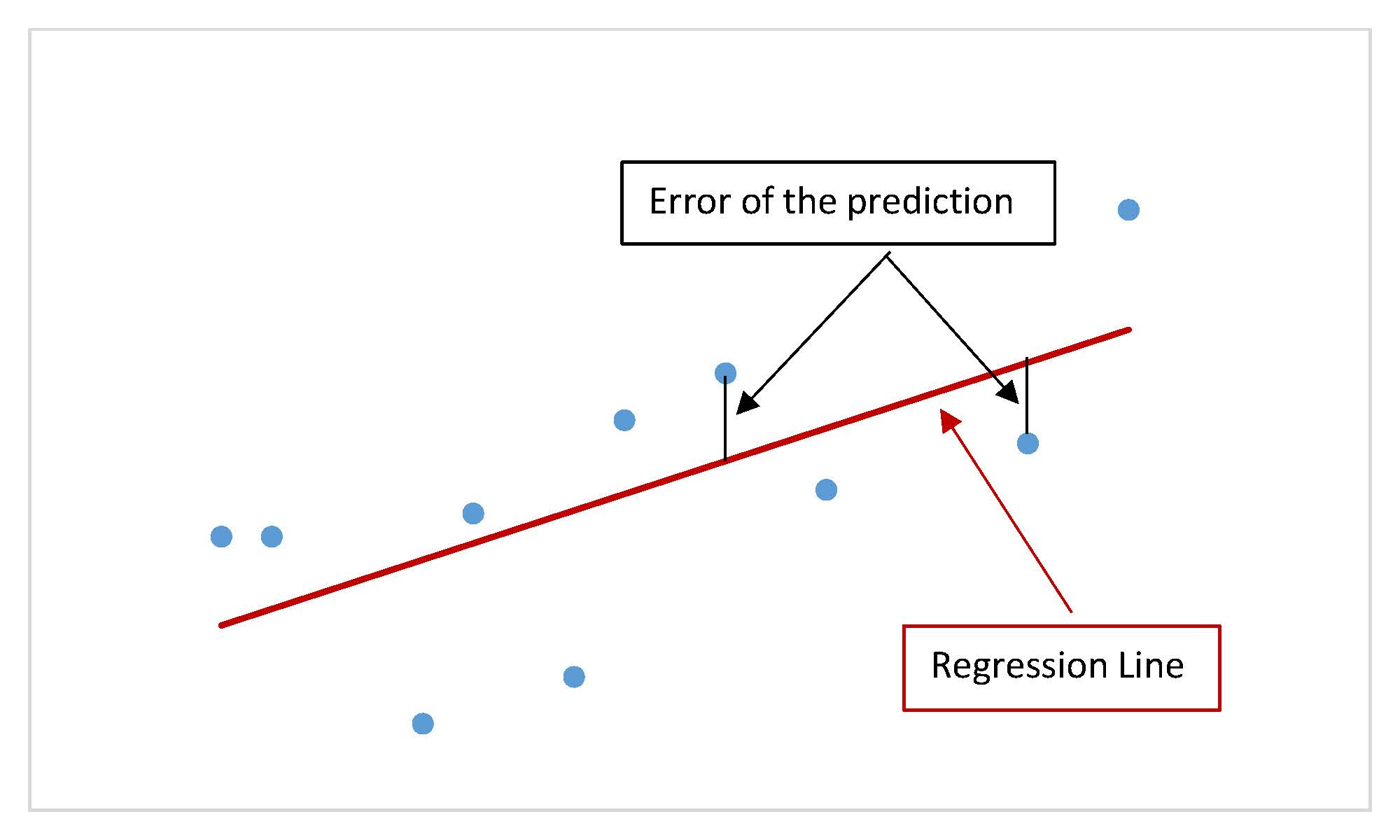
The standard error of the estimate, denoted [latex]s_e[/latex], is a measure of the standard deviation of the errors in a regression model. The standard error of the estimate is a measure of the average deviation of the errors, the difference between the [latex]\hat{y}[/latex]-values predicted by the multiple regression model and the [latex]y[/latex]-values in the sample. The standard error of the estimate for the regression model is the standard deviation of the errors/residuals.
The value of [latex]s_e[/latex] tells us, on average, how much the dependent variable differs from the regression model based on the independent variables. When interpreting the standard error of the estimate, remember to be specific to the question, using the actual names of the dependent and independent variables, and include appropriate units. The units of the standard error of the estimate are the same as the units of the dependent variable.
The value of the standard error of the estimate for the regression model can be found in the regression summary table, which we learned how to generate in Excel in the previous section.
EXAMPLE
The human resources department at a large company wants to develop a model to predict an employee’s job satisfaction from the number of hours of unpaid work per week the employee does, the employee’s age, and the employee’s income. A sample of [latex]25[/latex] employees at the company is taken, and the data is recorded in the table below. The employee’s income is recorded in [latex]\$1000[/latex]s, and the job satisfaction score is out of [latex]10[/latex], with higher values indicating greater job satisfaction.
| Job Satisfaction | Hours of Unpaid Work per Week | Age | Income ([latex]\$1000[/latex]s) |
|---|---|---|---|
| 4 | 3 | 23 | 60 |
| 5 | 8 | 32 | 114 |
| 2 | 9 | 28 | 45 |
| 6 | 4 | 60 | 187 |
| 7 | 3 | 62 | 175 |
| 8 | 1 | 43 | 125 |
| 7 | 6 | 60 | 93 |
| 3 | 3 | 37 | 57 |
| 5 | 2 | 24 | 47 |
| 5 | 5 | 64 | 128 |
| 7 | 2 | 28 | 66 |
| 8 | 1 | 66 | 146 |
| 5 | 7 | 35 | 89 |
| 2 | 5 | 37 | 56 |
| 4 | 0 | 59 | 65 |
| 6 | 2 | 32 | 95 |
| 5 | 6 | 76 | 82 |
| 7 | 5 | 25 | 90 |
| 9 | 0 | 55 | 137 |
| 8 | 3 | 34 | 91 |
| 7 | 5 | 54 | 184 |
| 9 | 1 | 57 | 60 |
| 7 | 0 | 68 | 39 |
| 10 | 2 | 66 | 187 |
| 5 | 0 | 50 | 49 |
Previously, we found the multiple regression equation to predict the job satisfaction score from the other variables:
[latex]\begin{eqnarray*}\hat{y}&=&4.7993-0.3818x_1+0.0046x_2+0.0233x_3\\\\\hat{y}&=&\text{predicted job satisfaction score}\\x_1&=&\text{hours of unpaid work per week}\\x_2&=&\text{age}\\x_3&=&\text{income (\$1000s)}\end{eqnarray*}[/latex]
- Find the standard error of the estimate.
- Interpret the standard error of the estimate.
Solution
- The regression summary table generated by Excel is shown below:
SUMMARY OUTPUT Regression Statistics Multiple R 0.711779225 R Square 0.506629665 Adjusted R Square 0.436148189 Standard Error 1.585212784 Observations 25 ANOVA df SS MS F Significance F Regression 3 54.189109 18.06303633 7.18812504 0.001683189 Residual 21 52.770891 2.512899571 Total 24 106.96 Coefficients Standard Error t Stat P-value Lower 95% Upper 95% Intercept 4.799258185 1.197185164 4.008785216 0.00063622 2.309575344 7.288941027 Hours of Unpaid Work per Week -0.38184722 0.130750479 -2.9204269 0.008177146 -0.65375772 -0.10993671 Age 0.004555815 0.022855709 0.199329423 0.843922453 -0.04297523 0.052086864 Income ([latex]\$1000[/latex]s) 0.023250418 0.007610353 3.055103771 0.006012895 0.007423823 0.039077013 The standard error of the estimate for the regression model is in the top part of the table, under the Regression Statistics heading in the Standard Error row. The value of the standard error of the estimate is [latex]s_e=1.5852[/latex].
- On average, the job satisfaction score is [latex]1.5852[/latex] points away from the regression model based on the independent variables “hours of unpaid work per week,” “age,” and “income.”
NOTE
The standard error of the estimate for the regression model is located in the top part of the table under the Regression Statistics heading. You will notice another standard error column at the bottom in the rows corresponding to the independent variables. These standard errors in the bottom part of the table are not related to the standard error of the estimate. In fact, the standard errors in the independent variable rows are measures of the uncertainty around the estimate of the regression coefficient for each independent variable.
Exercises
- A local restaurant advocacy group wants to study the relationship between a restaurant’s average weekly profit, the restaurant’s seating capacity, and the average daily traffic that passes the restaurant’s location. The group took a sample of restaurants and recorded their average weekly profit (in [latex]\$1000[/latex]s), the seating restaurant’s seating capacity, and the average number of cars (in [latex]1000[/latex]s) that passes the restaurant’s location. The data is recorded in the following table:
Seating Capacity Traffic Count ([latex]1000[/latex]s) Weekly Net Profit ([latex]\$1000[/latex]s) 120 19 23.8 180 8 29.2 150 12 22 180 15 26.2 220 16 33.5 235 10 32 115 18 22.4 110 12 20.4 165 21 23.7 220 20 34.7 140 24 27.1 145 24 23.3 140 13 20.9 200 14 29.6 210 14 31.4 175 12 23.2 175 15 31.1 190 17 28.2 100 23 25.2 145 20 20.7 135 13 37.2 25 13 26.3 140 25 20 130 14 28.2 135 10 24.6 160 23 23.7 In Question 1 of Section 13.1, we found the regression model to predict the average weekly profit from other variables.
- Find the standard error of the estimate for the regression model.
- Interpret the standard error of the estimate.
Click to see Answer
- [latex]4.1675[/latex]
- On average, the average weekly profit differs by [latex]\$4,167.50[/latex] from the regression model based on seating capacity and traffic count.
- A local university wants to study the relationship between a student’s GPA, the average number of hours they spend studying each night, and the average number of nights they go out each week. The university took a sample of students and recorded the following data:
GPA Average Number of Hours Spent Studying Each Night Average Number of Nights Go Out Each Week 3.72 5 1 3.88 3 1 3.67 2 1 3.87 3 4 2.49 1 4 1.29 1 2 1.01 2 4 2.12 1 1 1.9 1 5 3.42 3 2 1.33 1 4 1.07 0 2 2.75 3 1 3.82 4 1 3.91 5 0 2.25 2 3 2.06 1 5 2.92 3 2 3.06 3 1 3.65 2 2 3.69 4 1 In Question 2 of Section 13.1, we found the regression model to predict GPA from other variables.
- Find the standard error of the estimate for the regression model.
- Interpret the standard error of the estimate.
Click to see Answer
- [latex]0.6613[/latex]
- On average, GPA differs by [latex]0.6613[/latex] from the regression model based on the average number of hours spent studying a night and the average number of nights a student goes out each week.
- A very large company wants to study the relationship between the salaries of employees in management positions, their age, the number of years the employee spent in college, and the number of years the employee has been with the company. A sample of management employees is taken, and the data is recorded below:
Age Years of College Years with Company Salary ([latex]\$1000[/latex]s) 60 8 29 317.3 33 3 5 97.3 57 6 27 263.1 32 4 5 101.3 31 6 3 114.2 61 8 19 350.4 41 7 8 146.9 35 4 2 91.7 51 6 21 198.2 50 8 10 196.5 57 5 15 105.7 49 6 18 118.3 62 7 27 305.2 52 8 26 239.9 39 4 8 145.9 42 7 5 175.4 62 4 24 219.4 60 4 22 202.1 65 3 21 196.3 40 4 10 143.9 62 6 29 408.7 53 7 5 145.2 48 8 5 175.1 61 5 6 152.7 38 7 3 99.7 40 7 12 174.9 45 7 7 149.2 58 7 14 282.8 38 4 3 95.7 41 5 18 232.8 In Question 3 of Section 13.1, we found the regression model to predict salary from other variables.
- Find the standard error of the estimate for the regression model.
- Interpret the standard error of the estimate.
Click to see Answer
- [latex]45.24522[/latex]
- On average, salary differs by [latex]\$45,255.22[/latex] from the regression model based on age, years of college, and years with the company.
“13.3 Standard Error of the Estimate” and “13.8 Exercises” from Introduction to Statistics by Valerie Watts is licensed under a Creative Commons Attribution-NonCommercial-ShareAlike 4.0 International License, except where otherwise noted.
