12.4 The Regression Equation
LEARNING OBJECTIVES
- Find the equation of the line-of-best fit.
- Use the line-of-best-fit to make predictions.
We often want to use the values of the independent variable to make predictions about the value of the dependent variable. For example, we might want to use the amount a business spends on advertising each quarter to make a prediction about the revenue the business will generate that quarter. When a linear relationship exists between an independent and dependent variable, we can build a linear model of that relationship, and then we can use that model to make predictions about the dependent variable.
Simple linear regression is a modelling technique in which the linear relationship between one independent variable [latex]x[/latex] and one dependent variable [latex]y[/latex] is approximated by a straight line, called the line-of-best-fit or least squares line. It is important to note that the line-of-best-fit only models the linear relationship between the independent and dependent variables.
The equation for the regression line is
[latex]\begin{eqnarray*}\hat{y}&=&b_0+b_1x\\\\\hat{y}&=&\text{predicted value of }y\\x&=&\text{value of the independent variable}\\b_0&=&y\text{-interecept of the line}\\b_1&=&\text{slope of the line}\end{eqnarray*}[/latex]
The value of [latex]\hat{y}[/latex] is the estimated value of [latex]y[/latex]. It is the value of [latex]y[/latex] obtained using the regression line. The value of [latex]\hat{y}[/latex] is not generally equal to the value of [latex]y[/latex] from the sample data. The values for the slope [latex]b_1[/latex] and the [latex]y[/latex]-intercept [latex]b_0[/latex] in the line-of-best-fit are calculated using the sample data and the least squares method. Although there are formulas to calculate the values of the slope and [latex]y[/latex]-intercept in the regression line, we will calculate the slope and [latex]y[/latex]-intercept using the built-in functions in Excel.
What does the slope of the linear regression equation tell us?
- The slope of the line-of-best-fit [latex]b_1[/latex] and the correlation coefficient [latex]r[/latex] have the same sign. That is, [latex]b_1[/latex] and [latex]r[/latex] are either both positive or both negative.
- The slope [latex]b_1[/latex] of the regression equation tells us how the dependent variable [latex]y[/latex] changes for a one-unit increase in the independent variable [latex]x[/latex].
- When interpreting the slope, be specific to the context of the question, using the actual names of the variable and correct units.
What does the [latex]y[/latex]-intercept of the linear regression equation tell us?
- The [latex]y[/latex]-intercept [latex]b_0[/latex] of the line-of-best-fit is the predicted value of the dependent variable [latex]y[/latex] when [latex]x=0[/latex].
- When interpreting the [latex]y[/latex]-intercept, be specific to the context of the question, using the actual names of the variable and correct units.
CALCULATING THE SLOPE AND [latex]{\color{white}{y}}[/latex]-INTERCEPT OF THE LINEAR REGRESSION EQUATION IN EXCEL
To calculate the slope of the linear regression equation, use the slope(array for y’s, array for x’s) function.
- For array for y’s, enter the cell array containing the dependent variable [latex]y[/latex] data.
- For array for x’s, enter the cell array containing the independent variable [latex]x[/latex] data.
Visit the Microsoft page for more information about the slope function.
To calculate the [latex]y[/latex]-intercept of the linear regression equation, use the intercept(array for y’s, array for x’s) function.
- For array for y’s, enter the cell array containing the dependent variable [latex]y[/latex] data.
- For array for x’s, enter the cell array containing the independent variable [latex]x[/latex] data.
Visit the Microsoft page for more information about the intercept function.
NOTE
The order in which the data is entered into these functions is important. In both the slope and intercept functions, the data for the dependent variable is entered in the first array, and the data for the independent variable is entered in the second array. The output from the slope and intercept function will be different when the order of the inputs are switched.
EXAMPLE
A statistics professor wants to study the relationship between a student’s score on the third exam in the course and their final exam score. The professor took a random sample of [latex]11[/latex] students and recorded their third exam score (out of [latex]80[/latex]) and their final exam score (out of [latex]200[/latex]). The results are recorded in the table below. The professor wants to develop a linear regression model to predict a student’s final exam score from the third exam score.
| Student | Third Exam Score | Final Exam Score |
|---|---|---|
| 1 | 65 | 175 |
| 2 | 67 | 133 |
| 3 | 71 | 185 |
| 4 | 71 | 163 |
| 5 | 66 | 126 |
| 6 | 75 | 198 |
| 7 | 67 | 153 |
| 8 | 70 | 163 |
| 9 | 71 | 159 |
| 10 | 69 | 151 |
| 11 | 69 | 159 |
- Find the equation for the line-of-best-fit.
- Interpret the slope of the line-of-best fit.
Solution
- Because we want to predict the final exam score from the third exam score, the independent variable [latex]x[/latex] is the third exam score, and the dependent variable [latex]y[/latex] is the final exam score. Enter the data into an Excel spreadsheet. For this example, suppose we entered the data (without the column headings) so that the student column is in column A from A1 to A11, the third exam score is in column B from B1 to B11, and the final exam score is in column C from C1 to C11.
Function slope Field 1 C1:C11 Field 2 B1:B11 Answer 4.83 Function intercept Field 1 C1:C11 Field 2 B1:B11 Answer -173.51 The equation for the line-of-best-fit is [latex]\hat{y}=-173.51+4.83x[/latex] where [latex]x[/latex] is the third exam score and [latex]\hat{y}[/latex] is the (predicted) final exam score.
The graph below shows the scatter diagram with the line-of-best fit.
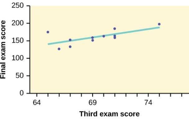
- The slope is [latex]b_1=4.83[/latex]. Interpretation: For a one-point increase in the score on the third exam, the final exam score increases by [latex]4.83[/latex] points.
NOTE
- When writing down the linear regression equation, remember to define what the variables represent in the context of the question. That is, state what [latex]x[/latex] and [latex]\hat{y}[/latex] represent in relation to the question.
- When writing down the interpretation of the slope, remember to be specific to the question using the actual names of the independent and dependent variables and appropriate units.
Making Predictions with the Linear Regression Equation
Given a specific value of the independent variable [latex]x[/latex], the linear regression equation may be used to predict/estimate the value of the dependent variable [latex]y[/latex]. To make predictions, the following conditions must be met:
- There must be a linear relationship between the variables. The stronger the linear relationship, the better the prediction will be.
- The linear regression equation is only valid to predict the values of the dependent variable. That is, we may only use the equation to solve for [latex]\hat{y}[/latex] for a given value of [latex]x[/latex], and not the other way around.
- The linear regression equation should only be used to make predictions for [latex]y[/latex] for values of [latex]x[/latex] within the domain of the [latex]x[/latex] values in the sample data used to construct the regression equation. The regression equation does not provide reliable predictions for values of [latex]x[/latex] that fall outside the domain of the [latex]x[/latex] values in the sample data.
EXAMPLE
A statistics professor wants to study the relationship between a student’s score on the third exam in the course and their final exam score. The professor took a random sample of [latex]11[/latex] students and recorded their third exam score (out of [latex]80[/latex]) and their final exam score (out of [latex]200[/latex]). The results are recorded in the table below. The professor developed the linear regression model [latex]\hat{y}=-173.51+4.83x[/latex] to predict a student’s final exam score ([latex]\hat{y}[/latex]) from a student’s third exam score ([latex]x[/latex]).
| Student | Third Exam Score | Final Exam Score |
|---|---|---|
| 1 | 65 | 175 |
| 2 | 67 | 133 |
| 3 | 71 | 185 |
| 4 | 71 | 163 |
| 5 | 66 | 126 |
| 6 | 75 | 198 |
| 7 | 67 | 153 |
| 8 | 70 | 163 |
| 9 | 71 | 159 |
| 10 | 69 | 151 |
| 11 | 69 | 159 |
- What is the professor’s final exam prediction for a student who scored [latex]66[/latex] on the third exam?
- What is the professor’s final exam prediction for a student who scored [latex]73[/latex] on the third exam?
- Should the professor use the linear regression model to predict the final exam score for a student who scored [latex]80[/latex] on the third exam? Why?
Solution
- Substitute [latex]x=66[/latex] into the linear regression equation:
[latex]\begin{eqnarray*}\\\hat{y}&=&-173.51+4.83\times 66\\&=&145.27\end{eqnarray*}[/latex]
A student who scored [latex]66[/latex] on the third exam has a predicted score of [latex]145.27[/latex] on the final exam.
- Substitute [latex]x=73[/latex] into the linear regression equation:
[latex]\begin{eqnarray*}\\\hat{y}&=&-173.51+4.83\times 73\\&=&179.08\end{eqnarray*}[/latex]
A student who scored [latex]73[/latex] on the third exam has a predicted score of [latex]179.08[/latex] on the final exam.
- The [latex]x[/latex] values (third exam score) in the sample data are between [latex]65[/latex] and [latex]75[/latex]. An [latex]x[/latex] value of [latex]80[/latex] is outside the domain of the observed [latex]x[/latex] values in the data. So, we cannot reliably predict the final exam score for a student who scored [latex]80[/latex] on the third exam. Of course, it is possible to enter [latex]x=80[/latex] into the linear regression equation and calculate the corresponding value of [latex]\hat{y}[/latex], but this value is not a reliable prediction. If we calculate out the value of [latex]\hat{y}[/latex] in the regression equation for [latex]x=80[/latex], we get [latex]\hat{y}=212.89[/latex], a value that makes no sense in the context of the question because the maximum score on the final exam is [latex]200[/latex].
NOTES
- The values obtained for the linear regression equation are predictions only. Here, [latex]145.27[/latex] is the predicted final exam score for a student who scored [latex]66[/latex] on the third exam. This does not mean that a student who actually scored [latex]66[/latex] on the third exam will score [latex]145.27[/latex] on the final exam.
- Remember that the linear regression equation only gives reliable predictions for values of [latex]x[/latex] that fall within the domain of [latex]x[/latex] values in the sample data.
TRY IT
SCUBA divers have maximum dive times they cannot exceed when going to different depths. The data in the table below shows different depths with the maximum dive times in minutes.
| Depth (in feet) | Maximum Dive Time (in minutes) |
|---|---|
| 50 | 80 |
| 60 | 55 |
| 70 | 45 |
| 80 | 35 |
| 90 | 25 |
| 100 | 22 |
- Find the linear regression equation to predict the maximum dive time from the depth.
- Interpret the slope of the regression equation found in part 1.
- Predict the maximum dive time for a depth of [latex]75[/latex] feet.
Click to see Solution
- [latex]\displaystyle{\hat{y}=127.24-1.11x}[/latex] where [latex]x[/latex] is the depth in feet and [latex]\hat{y}[/latex] is the (predicted) maximum dive time in minutes.
- For each one-foot increase in depth, the maximum dive time decreases by [latex]1.11[/latex] minutes.
- [latex]\displaystyle{\hat{y}=127.24-1.11\times 75=43.99\text{ minutes}}[/latex]
Errors and The Least Squares Method
The difference between the actual value of the dependent variable [latex]y[/latex] (in the sample date) and the predicted value of the dependent variable [latex]\hat{y}[/latex] obtained from the linear regression equation is called the error or residual.
[latex]\begin{eqnarray*}\text{Error}&=&\text{Actual Value}-\text{Predicted Value}\\&=&y-\hat{y}\end{eqnarray*}[/latex]
Graphically, the absolute value of the error is the vertical distance between the actual value of [latex]y[/latex] (the point on the scatter diagram) and the predicted value of [latex]\hat{y}[/latex] (the point on the linear regression line). In other words, the absolute value of the error measures the vertical distance between the actual data point and the line.
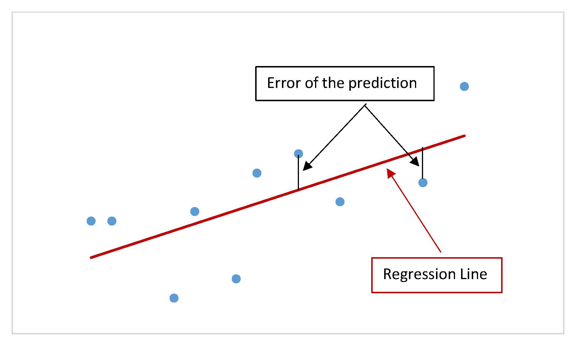
The slope and [latex]y[/latex]-intercept for the linear regression equation are generated using the errors and the least squares method. The idea behind finding the line of best fit is based on the assumption that the data are scattered about a straight line. For any line, the errors can be calculated, squared, and then these squared errors can be added up. Of all of the possible lines, the line-of-best-fit is the one line that minimizes this sum of the squared errors. Any other line will have a higher sum of the squared errors compared to the sum of the squared errors for the line-of-best-fit.
Video: “Basic Excel Business Analytics #46: Slope & Intercept for Estimated Simple Liner Regression Equation” by excelisfun [18:29] is licensed under the Standard YouTube License.Transcript and closed captions available on YouTube.
Exercises
- What is the process through which we can calculate a line that goes through a scatter plot with a linear pattern?
Click to see Answer
Simple linear regression
- An electronics retailer used regression to find a simple model to predict sales growth in the first quarter of the new year (January through March). The model is good for [latex]90[/latex] days, where [latex]x[/latex] is the day. The model can be written as [latex]\hat{y}=101.32+2.48x[/latex] where [latex]\hat{y}[/latex] is in thousands of dollars.
- What would you predict the sales to be on day [latex]60[/latex]?
- What would you predict the sales to be on day [latex]90[/latex]?
Click to see Answer
- [latex]\$250,120[/latex]
- [latex]\$342,520[/latex]
- A landscaping company is hired to mow the grass for several large properties. The total area of the properties combined is [latex]1,345[/latex] acres. The rate at which one person can mow is [latex]\hat{y}=1350–1.2x[/latex] where [latex]x[/latex] is the number of hours and [latex]\hat{y}[/latex] represents the number of acres left to mow.
- How many acres will be left to mow after [latex]20[/latex] hours of work?
- How many acres will be left to mow after [latex]100[/latex] hours of work?
- How many hours will it take to mow all of the lawns?
Click to see Answer
- [latex]1,326[/latex]
- [latex]1,230[/latex]
- [latex]1,125[/latex]
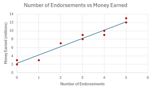
- In a random sample of ten professional athletes, the number of endorsements the player has and the amount of money (in millions of dollars) the player earns are recorded in the table below.
Player Number of Endorsements Money Earned (in millions) 1 0 2 2 3 8 3 2 7 4 1 3 5 5 13 6 5 12 7 4 9 8 3 9 9 0 3 10 4 10 - Which variable is the independent variable, and which variable is the dependent variable?
- Use regression to find the equation for the line-of-best fit.
- Draw the scatter diagram for this data and include the line-of-best fit on the scatter diagram.
- What is the slope of the line of best fit? What does it represent?
- What is the [latex]y[/latex]-intercept of the line-of-best-fit? What does it represent?
- Predict the amount of money a professional athlete earns if they have [latex]2[/latex] endorsements.
Click to see Answer
- Independent: number of endorsements; Dependent: money earned
- [latex]\hat{y}=2.234+1.988x[/latex] where [latex]x[/latex] is the number of endorsements and [latex]\hat{y}[/latex] is the money earned.
- [latex]1.988[/latex]. For each extra endorsement an athlete has, the amount of money earned increases by [latex]\$1,988,000[/latex].
- [latex]2.234[/latex]. A player with [latex]0[/latex] endorsements will earn [latex]\$2,234,000[/latex].
- [latex]\$6,208,723[/latex]
- The table below gives the percentage of workers who are paid hourly rates for the years 1979 to 1992. (Note: for identification of the independent and dependent variables, refer back to Question 7 in Section 12.2.)
Year Percent of Workers Paid Hourly Rates 1979 61.2 1980 60.7 1981 61.3 1982 61.3 1983 61.8 1984 61.7 1985 61.8 1986 62.0 1987 62.7 1990 62.8 1992 62.9 - Find the linear regression equation.
- Interpret the slope of the linear regression equation.
- What is the estimated percentage of workers paid hourly rates in 1988?
Click to see Answer
- [latex]\hat{y}=-266.89+0.17x[/latex] where [latex]x[/latex] is the year and [latex]\hat{y}[/latex] is the percent of workers paid an hourly rate.
- For each additional year, the percent of workers paid an hourly rate increases by [latex]0.17\%[/latex].
- [latex]62.42\%[/latex]
- The table below contains real data for the first two decades of AIDS cases. (Note: for identification of the independent and dependent variables, refer back to Question 1 in Section 12.2.)
Year Number of AIDS Cases 1981 319 1982 1,170 1983 3,076 1984 6,240 1985 11,776 1986 19,032 1987 28,564 1988 35,447 1989 42,674 1990 48,634 1991 59,660 1992 78,530 1993 78,834 1994 71,874 1995 68,505 1996 59,347 1997 47,149 1998 38,393 1999 25,174 2000 25,522 2001 25,643 2002 26,464 - Find the linear regression equation.
- Interpret the slope of the linear regression equation.
- What is the predicted number of diagnosed cases for the year 1985?
- What is the predicted number of diagnosed cases for the year 1970? Why does this answer not make sense?
Click to see Answer
- [latex]\hat{y}=-3,448,225.05+1749.78x[/latex] where [latex]x[/latex] is the year and [latex]\hat{y}[/latex] is the number of AIDS cases.
- For each additional year, the number of AIDS cases increases by [latex]1749.78[/latex].
- [latex]25,082.22[/latex]
- [latex]-1164.43[/latex]. The number of AIDS cases is a count and so must be positive.
- Recently, the annual number of driver deaths per [latex]100,000[/latex] for the selected age groups was as shown in the table below. (Note: for identification of the independent and dependent variables, refer back to Question 8 in Section 12.2.)
Age Number of Driver Deaths per [latex]100,000[/latex] 17.5 38 22 36 29.5 24 44.5 20 64.5 18 80 28 - Calculate the least squares (best–fit) line.
- Interpret the slope of the least squares line.
- Predict the number of driver deaths per [latex]100,000[/latex] for people aged 40.
Click to see Answer
- [latex]\hat{y}=35.58-0.19x[/latex] where [latex]x[/latex] is the age and [latex]\hat{y}[/latex] is the number of driver deaths per 100,000.
- For each additional year of age, the number of driver deaths per [latex]100,000[/latex] decreases by [latex]0.19[/latex].
- [latex]27.91[/latex]
- The table below shows the life expectancy for an individual born in the United States in certain years. (Note: for identification of the independent and dependent variables, refer back to Question 9 in Section 12.2.)
Year of Birth Life Expectancy 1930 59.7 1940 62.9 1950 70.2 1965 69.7 1973 71.4 1982 74.5 1987 75 1992 75.7 2010 78.7 - Find the linear regression equation.
- Interpret the slope of the linear regression equation.
- What is the estimated life expectancy for someone born in 1950? Why doesn’t this value match the life expectancy given in the table for 1950?
- What is the estimated life expectancy for someone born in 1982?
- Using the regression equation, find the estimated life expectancy for someone born in 1850. Is this an accurate estimate for that year? Explain why or why not.
Click to see Answer
- [latex]\hat{y}=-377.24+0.23x[/latex] where [latex]x[/latex] is the year and [latex]\hat{y}[/latex] is life expectancy.
- For each additional year, the life expectancy increases by [latex]0.23[/latex] years.
- [latex]66.34[/latex]. This is the value predicted by the model, which generally does not equal the actual value given in the data.
- [latex]73.62[/latex] years
- [latex]43.59[/latex] years. This is not an accurate estimate because the year 1850 is outside of the domain of the values of the independent variable provided in the data.
- The height (sidewalk to roof) of notable tall buildings in America is compared to the number of stories of the building (beginning at street level). (Note: for identification of the independent and dependent variables, refer back to Question 10 in Section 12.2.)
Height (in feet) Number of Stories 1,050 57 428 28 362 26 529 40 790 60 401 22 380 38 1,454 110 1,127 100 700 46 - Find the linear regression equation.
- Interpret the slope of the linear regression equation.
- What is the estimated height for a 32-story building?
- What is the estimated height for a 94-story building?
- Using the regression equation, find the estimated height for a 6-story building. Is this an accurate estimate for the height of a 6-story building? Explain why or why not.
Click to see Answer
- [latex]\hat{y}=102.43+11.76x[/latex] where [latex]x[/latex] is the number of stories and [latex]\hat{y}[/latex] is the height.
- For each additional story, the height of the building increases by [latex]11.76[/latex] feet.
- [latex]478.70[/latex] feet
- [latex]1207.73[/latex] feet
- [latex]172.98[/latex] feet. This is not accurate because [latex]6[/latex] is outside the domain of the independent variable given in the data.
- The following table shows data on average per capita wine consumption and heart disease rate in a random sample of 10 countries. (Note: for identification of the independent and dependent variables, refer back to Question 11 in Section 12.2.)
Per Capita Yearly Wine Consumption in Liters Per Capita Death from Heart Disease 2.5 221 3.9 167 2.9 131 2.4 191 2.9 220 0.8 297 9.1 71 2.7 172 0.8 211 0.7 300 - Find the linear regression equation.
- Interpret the slope of the linear regression equation.
- What is the predicted per capita heart disease rate for a per capita yearly wine consumption of [latex]2[/latex] litres?
Click to see Answer
- [latex]\hat{y}=266.63-23.88x[/latex] where [latex]x[/latex] is the per capita yearly wine consumption and [latex]\hat{y}[/latex] is the per capita deaths from heart disease.
- For each additional litre of wine consumed per year, the number of deaths from heart disease decreases by [latex]23.88[/latex].
- [latex]218.87[/latex]
- The following table consists of one student athlete’s time (in minutes) to swim 2000 meters and the student’s heart rate (beats per minute) after swimming on a random sample of 10 days. (Note: for identification of the independent and dependent variables, refer back to Question 12 in Section 12.2.)
Swim Time Heart Rate 34.12 144 35.72 152 34.72 124 34.05 140 34.13 152 35.73 146 36.17 128 35.57 136 35.37 144 35.57 148 - Find the linear regression equation.
- Interpret the slope of the linear regression equation.
- What is the estimated heart rate for a swim time of [latex]34.75[/latex] minutes?
Click to see Answer
- [latex]\hat{y}=193.88-1.49x[/latex] where [latex]x[/latex] is the swim time and [latex]\hat{y}[/latex] is the heart rate.
- For each additional minute of swim time, the heart rate decreases by [latex]1.49[/latex] beats per minute.
- [latex]141.95[/latex] bpm
“12.5 The Regression Equation” and “12.8 Exercises” from Introduction to Statistics by Valerie Watts is licensed under a Creative Commons Attribution-NonCommercial-ShareAlike 4.0 International License, except where otherwise noted.
