8.5 Hypothesis Tests for a Population Mean with Unknown Population Standard Deviation
LEARNING OBJECTIVES
- Conduct and interpret hypothesis tests for a population mean with unknown population standard deviation.
Some notes about conducting a hypothesis test:
- The null hypothesis [latex]H_0[/latex] is always an “equal to.” The null hypothesis is the original claim about the population parameter.
- The alternative hypothesis [latex]H_a[/latex] is a “less than,” “greater than,” or “not equal to.” The form of the alternative hypothesis depends on the context of the question.
- The form of the alternative hypothesis tells us if the test is left-tail, right-tail, or two-tail. The alternative hypothesis is the key to conducting the test and finding the correct [latex]p-\text{value}[/latex].
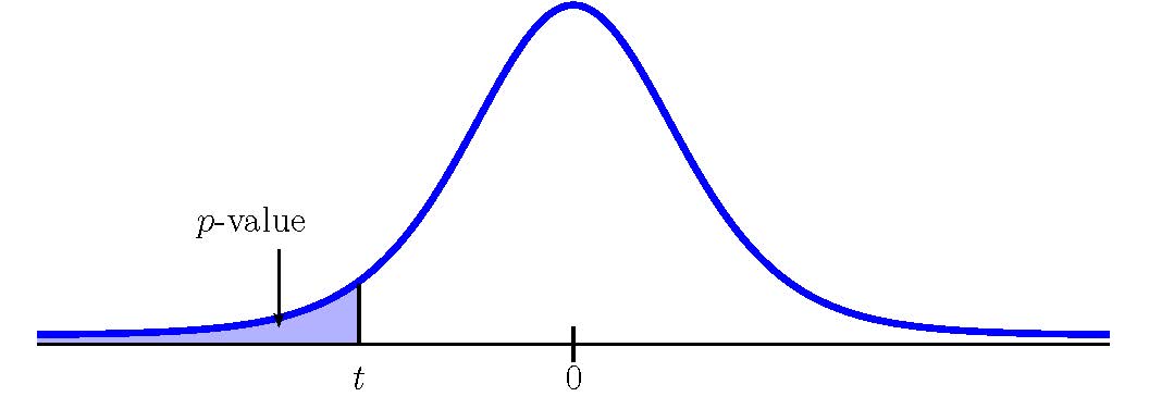
- If the alternative hypothesis is a “less than”, then the test is left-tail. The [latex]p-\text{value}[/latex] is the area in the left-tail of the distribution.
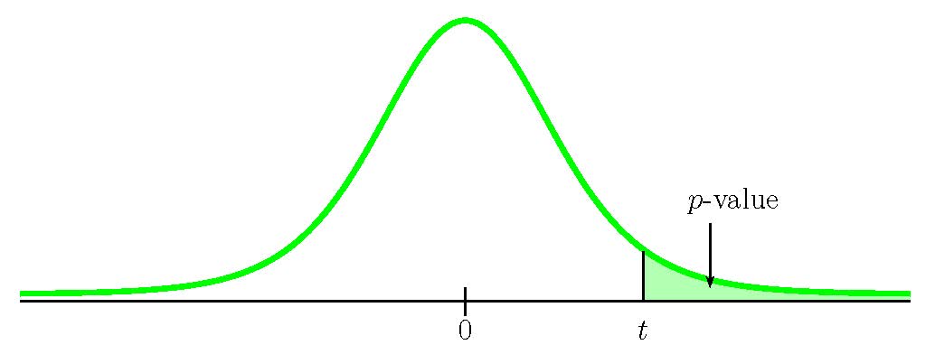
- If the alternative hypothesis is a “greater than”, then the test is right-tail. The [latex]p-\text{value}[/latex] is the area in the right-tail of the distribution.
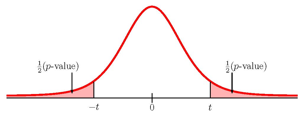
- If the alternative hypothesis is a “not equal to”, then the test is two-tail. The [latex]p-\text{value}[/latex] is the sum of the area in the two-tails of the distribution. Each tail represents exactly half of the [latex]p-\text{value}[/latex].
- Think about the meaning of the [latex]p-\text{value}[/latex]. A data analyst (and anyone else) should have more confidence that they made the correct decision to reject the null hypothesis with a smaller [latex]p-\text{value}[/latex] (for example, [latex]0.001[/latex] as opposed to [latex]0.04[/latex]) even if using a significance level of [latex]0.05[/latex]. Similarly, for a large [latex]p-\text{value}[/latex] such as [latex]0.4[/latex], as opposed to a [latex]p-\text{value}[/latex] of [latex]0.056[/latex] (a significance level of [latex]0.05[/latex] is less than either number), a data analyst should have more confidence that they made the correct decision in not rejecting the null hypothesis. This makes the data analyst use judgment rather than mindlessly applying rules.
- The significance level must be identified before collecting the sample data and conducting the test. Generally, the significance level will be included in the question. If no significance level is given, a common standard is to use a significance level of [latex]5\%[/latex].
- An alternative approach for hypothesis testing is to use what is called the critical value approach. In this book, we will only use the [latex]p-\text{value}[/latex] approach. Some of the videos below may mention the critical value approach, but this approach will not be used in this book.
Conducting a Hypothesis Test for a Population Mean with Unknown Population Standard Deviation
Follow these steps to perform a hypothesis test for a population mean with unknown population standard deviation:
- Write down the null and alternative hypotheses in terms of the population mean [latex]\mu[/latex]. Include appropriate units with the values of the mean.
- Use the form of the alternative hypothesis to determine if the test is left-tailed, right-tailed, or two-tailed.
- Collect the sample information for the test and identify the significance level [latex]\alpha[/latex].
- When the population standard deviation is unknown, the [latex]p-\text{value}[/latex] is the area in the corresponding tail of the [latex]t[/latex]-distribution with:
[latex]\begin{eqnarray*}t&=&\frac{\overline{x}-\mu}{\frac{s}{\sqrt{n}}}\\\\df&=&n-1\\\\\end{eqnarray*}[/latex]
- Compare the [latex]p-\text{value}[/latex] to the significance level and state the outcome of the test.
- If [latex]p-\text{value}\leq\alpha[/latex], reject [latex]H_0[/latex] in favour of [latex]H_a[/latex].
- The results of the sample data are significant. There is sufficient evidence to conclude that the null hypothesis [latex]H_0[/latex] is an incorrect belief and that the alternative hypothesis [latex]H_a[/latex] is most likely correct.
- If [latex]p-\text{value}\gt\alpha[/latex], do not reject [latex]H_0[/latex].
- The results of the sample data are not significant. There is not sufficient evidence to conclude that the alternative hypothesis [latex]H_a[/latex] may be correct.
- If [latex]p-\text{value}\leq\alpha[/latex], reject [latex]H_0[/latex] in favour of [latex]H_a[/latex].
- Write down a concluding sentence specific to the context of the question.
USING EXCEL TO CALCULE THE [latex]\color{white}{p-\text{value}}[/latex] FOR A HYPOTHESIS TEST ON A POPULATION MEAN WITH UNKNOWN POPULATION STANDARD DEVIATION
The [latex]p-\text{value}[/latex] for a hypothesis test on a population mean is the area in the tail(s) of the distribution of the sample mean. When the population standard deviation is unknown, use the [latex]t[/latex]-distribution to find the [latex]p-\text{value}[/latex].
If the [latex]p-\text{value}[/latex] is the area in the left-tail:
- Use the t.dist function to find the [latex]p-\text{value}[/latex]. In the t.dist(t-score, degrees of freedom, logic operator) function:
- For t-score, enter the value of [latex]t[/latex] calculated from [latex]\displaystyle{t=\frac{\overline{x}-\mu}{\frac{s}{\sqrt{n}}}}[/latex].
- For degrees of freedom, enter the degrees of freedom for the [latex]t[/latex]-distribution [latex]n-1[/latex].
- For the logic operator, enter true. Note: Because we are calculating the area under the curve, we always enter true for the logic operator.
- The output from the t.dist function is the area under the [latex]t[/latex]-distribution to the left of the entered [latex]t[/latex]-score.
- Visit the Microsoft page for more information about the t.dist function.
If the [latex]p-\text{value}[/latex] is the area in the right-tail:
- Use the t.dist.rt function to find the [latex]p-\text{value}[/latex]. In the t.dist.rt(t-score, degrees of freedom) function:
- For t-score, enter the value of [latex]t[/latex] calculated from [latex]\displaystyle{t=\frac{\overline{x}-\mu}{\frac{s}{\sqrt{n}}}}[/latex].
- For degrees of freedom, enter the degrees of freedom for the [latex]t[/latex]-distribution [latex]n-1[/latex].
- The output from the t.dist.rt function is the area under the [latex]t[/latex]-distribution to the right of the entered [latex]t[/latex]-score.
- Visit the Microsoft page for more information about the t.dist.rt function.
If the [latex]p-\text{value}[/latex] is the sum of area in the tails:
- Use the t.dist.2t function to find the [latex]p-\text{value}[/latex]. In the t.dist.2t(t-score, degrees of freedom) function:
- For t-score, enter the absolute value of [latex]t[/latex] calculated from [latex]\displaystyle{t=\frac{\overline{x}-\mu}{\frac{s}{\sqrt{n}}}}[/latex]. Note: In the t.dist.2t function, the value of the [latex]t[/latex]-score must be a positive number. If the [latex]t[/latex]-score is negative, enter the absolute value of the [latex]t[/latex]-score into the t.dist.2t function.
- For degrees of freedom, enter the degrees of freedom for the [latex]t[/latex]-distribution [latex]n-1[/latex].
- The output from the t.dist.2t function is the sum of areas in the tails under the [latex]t[/latex]-distribution.
- Visit the Microsoft page for more information about the t.dist.2t function.
EXAMPLE
Statistics students believe that the mean score on the first statistics test is [latex]65[/latex]. A statistics instructor thinks the mean score is higher than [latex]65[/latex]. He samples ten statistics students and obtains the following scores:
| Mean Scores | ||||
|---|---|---|---|---|
| [latex]65[/latex] | [latex]67[/latex] | [latex]66[/latex] | [latex]68[/latex] | [latex]72[/latex] |
| [latex]65[/latex] | [latex]70[/latex] | [latex]63[/latex] | [latex]63[/latex] | [latex]71[/latex] |
The instructor performs a hypothesis test using a [latex]1\%[/latex] level of significance. The test scores are assumed to be from a normal distribution.
Solution
Hypotheses:
[latex]\begin{eqnarray*}H_0:&&\mu=65\\H_a:&&\mu\gt 65\end{eqnarray*}[/latex]
[latex]p-\text{value}[/latex]:
From the question, we have [latex]n=10[/latex], [latex]\overline{x}=67[/latex], [latex]s=3.1972...[/latex] and [latex]\alpha=0.01[/latex].
This is a test on a population mean where the population standard deviation is unknown (we only know the sample standard deviation [latex]s=3.1972...[/latex]). So we use a [latex]t[/latex]-distribution to calculate the [latex]p-\text{value}[/latex]. Because the alternative hypothesis is a [latex]\gt[/latex], the [latex]p-\text{value}[/latex] is the area in the right-tail of the distribution.
To use the t.dist.rt function, we need to calculate out the [latex]t[/latex]-score:
[latex]\begin{eqnarray*}t&=&\frac{\overline{x}-\mu}{\frac{s}{\sqrt{n}}}\\&=&\frac{67-65}{\frac{3.1972...}{\sqrt{10}}}\\&=&1.9781...\end{eqnarray*}[/latex]
The degrees of freedom for the [latex]t[/latex]-distribution is [latex]n-1=10-1=9[/latex].
| Function | t.dist.rt |
|---|---|
| Field 1 | 1.9781…. |
| Field 2 | 9 |
| Answer | 0.0396 |
So the [latex]p-\text{value}=0.0396[/latex].
Conclusion:
Because [latex]p-\text{value}=0.0396\gt 0.01=\alpha[/latex], we do not reject the null hypothesis. At the [latex]1\%[/latex] significance level, there is not enough evidence to suggest that mean score on the test is greater than [latex]65[/latex].
NOTES
- The null hypothesis [latex]\mu=65[/latex] is the claim that the mean test score is [latex]65[/latex].
- The alternative hypothesis [latex]\mu\gt 65[/latex] is the claim that the mean test score is greater than [latex]65[/latex].
- Keep all of the decimals throughout the calculation (i.e. in the sample standard deviation, the [latex]t[/latex]-score, etc.) to avoid any round-off error in the calculation of the [latex]p-\text{value}[/latex]. This ensures that we get the most accurate value for the [latex]p-\text{value}[/latex].
- The [latex]p-\text{value}[/latex] is the area in the right-tail of the [latex]t[/latex]-distribution, to the right of [latex]t=1.9781...[/latex].
- The [latex]p-\text{value}[/latex] of [latex]0.0396[/latex] tells us that under the assumption that the mean test score is [latex]65[/latex] (the null hypothesis), there is a [latex]3.96\%[/latex] chance that the mean test score is [latex]65[/latex] or more. Compared to the [latex]1\%[/latex] significance level, this is a large probability, and so is likely to happen, assuming the null hypothesis is true. This suggests that the assumption that the null hypothesis is true is most likely correct, and so the conclusion of the test is to not reject the null hypothesis.
TRY IT
A company claims that the average change in the value of their stock is [latex]\$3.50[/latex] per week. An investor believes this average is too high. The investor records the changes in the company’s stock price over [latex]30[/latex] weeks and finds the average change in the stock price is [latex]\$2.60[/latex] with a standard deviation of [latex]\$1.80[/latex]. At the [latex]5\%[/latex] significance level, is the average change in the company’s stock price lower than the company claims?
Click to see Solution
Hypotheses:
[latex]\begin{eqnarray*}H_0:&&\mu=\$3.50\\H_a:&&\mu\lt\$3.50\end{eqnarray*}[/latex]
[latex]p-\text{value}[/latex]:
From the question, we have [latex]n=30[/latex], [latex]\overline{x}=2.6[/latex], [latex]s=1.8[/latex] and [latex]\alpha=0.05[/latex].
This is a test on a population mean where the population standard deviation is unknown (we only know the sample standard deviation [latex]s=1.8[/latex]). So we use a [latex]t[/latex]-distribution to calculate the [latex]p-\text{value}[/latex]. Because the alternative hypothesis is a [latex]\lt[/latex], the [latex]p-\text{value}[/latex] is the area in the left-tail of the distribution.
To use the t.dist function, we need to calculate out the [latex]t[/latex]-score:
[latex]\begin{eqnarray*}t&=&\frac{\overline{x}-\mu}{\frac{s}{\sqrt{n}}}\\&=&\frac{2.6-3.5}{\frac{1.8}{\sqrt{30}}}\\&=&-1.5699...\end{eqnarray*}[/latex]
The degrees of freedom for the [latex]t[/latex]-distribution is [latex]n-1=30-1=29[/latex].
| Function | t.dist |
|---|---|
| Field 1 | -1.5699…. |
| Field 2 | 29 |
| Field 3 | true |
| Answer | 0.0636 |
So the [latex]p-\text{value}=0.0636[/latex].
Conclusion:
Because [latex]p-\text{value}=0.0636\gt 0.05=\alpha[/latex], we do not reject the null hypothesis. At the [latex]5\%[/latex] significance level, there is not enough evidence to suggest that the average change in the stock price is lower than [latex]\$3.50[/latex].
NOTES
- The null hypothesis [latex]\mu=\$3.50[/latex] is the claim that the average change in the company’s stock is [latex]\$3.50[/latex] per week.
- The alternative hypothesis [latex]\mu\lt$3.50[/latex] is the claim that the average change in the company’s stock is less than [latex]\$3.50[/latex] per week.
- The [latex]p-\text{value}[/latex] is the area in the left-tail of the [latex]t[/latex]-distribution, to the left of [latex]t=-1.5699...[/latex].
- The [latex]p-\text{value}[/latex] of [latex]0.0636[/latex] tells us that under the assumption that the average change in the stock is [latex]\$3.50[/latex] (the null hypothesis), there is a [latex]6.36\%[/latex] chance that the average change is [latex]\$3.50[/latex] or less. Compared to the [latex]5\%[/latex] significance level, this is a large probability, and so is likely to happen, assuming the null hypothesis is true. This suggests that the assumption that the null hypothesis is true is most likely correct, and so the conclusion of the test is to not reject the null hypothesis. In other words, the company’s claim that the average change in their stock price is [latex]\$3.50[/latex] per week is most likely correct.
EXAMPLE
A paint manufacturer has their production line set-up so that the average volume of paint in a can is [latex]3.78[/latex] litres. The quality control manager at the plant believes that something has happened with the production, and the average volume of paint in the cans has changed. The quality control department takes a sample of [latex]100[/latex] cans and finds the average volume is [latex]3.62[/latex] litres with a standard deviation of [latex]0.7[/latex] litres. At the [latex]5\%[/latex] significance level, has the volume of paint in a can changed?
Solution
Hypotheses:
[latex]\begin{eqnarray*}H_0:&&\mu=3.78\text{ liters}\\H_a:&&\mu\neq 3.78\text{ liters}\end{eqnarray*}[/latex]
[latex]p-\text{value}[/latex]:
From the question, we have [latex]n=100[/latex], [latex]\overline{x}=3.62[/latex], [latex]s=0.7[/latex] and [latex]\alpha=0.05[/latex].
This is a test on a population mean where the population standard deviation is unknown (we only know the sample standard deviation [latex]s=0.7[/latex]). So we use a [latex]t[/latex]-distribution to calculate the [latex]p-\text{value}[/latex]. Because the alternative hypothesis is a [latex]\neq[/latex], the [latex]p-\text{value}[/latex] is the sum of the area in the tails of the distribution.
To use the t.dist.2t function, we need to calculate out the [latex]t[/latex]-score:
[latex]\begin{eqnarray*}t&=&\frac{\overline{x}-\mu}{\frac{s}{\sqrt{n}}}\\&=&\frac{3.62-3.78}{\frac{0.07}{\sqrt{100}}}\\&=&-2.2857...\end{eqnarray*}[/latex]
The degrees of freedom for the [latex]t[/latex]-distribution is [latex]n-1=100-1=99[/latex].
| Function | t.dist.2t |
|---|---|
| Field 1 | 2.2857…. |
| Field 2 | 99 |
| Answer | 0.0244 |
So the [latex]p-\text{value}=0.0244[/latex].
Conclusion:
Because [latex]p-\text{value}=0.0244\lt 0.05=\alpha[/latex], we reject the null hypothesis in favour of the alternative hypothesis. At the [latex]5\%[/latex] significance level, there is enough evidence to suggest that the average volume of paint in the cans has changed.
NOTES
- The null hypothesis [latex]\mu=3.78[/latex] is the claim that the average volume of paint in the cans is [latex]3.78[/latex].
- The alternative hypothesis [latex]\mu\neq 3.78[/latex] is the claim that the average volume of paint in the cans is not [latex]3.78[/latex].
- Keep all of the decimals throughout the calculation (i.e. in the [latex]t[/latex]-score) to avoid any round-off error in the calculation of the [latex]p-\text{value}[/latex]. This ensures that we get the most accurate value for the [latex]p-\text{value}[/latex].
- The [latex]p-\text{value}[/latex] is the sum of the area in the two tails. The output from the t.dist.2t function is exactly the sum of the area in the two tails, and so is the [latex]p-\text{value}[/latex] required for the test. No additional calculations are required.
- The t.dist.2t function requires that the value entered for the [latex]t[/latex]-score is positive. A negative [latex]t[/latex]-score entered into the t.dist.2t function generates an error in Excel. In this case, the value of the [latex]t[/latex]-score is negative, so we must enter the absolute value of this [latex]t[/latex]-score into field 1.
- The [latex]p-\text{value}[/latex] of [latex]0.0244[/latex] is a small probability compared to the significance level, and so is unlikely to happen, assuming the null hypothesis is true. This suggests that the assumption that the null hypothesis is true is most likely incorrect, and so the conclusion of the test is to reject the null hypothesis in favour of the alternative hypothesis. In other words, the average volume of paint in the cans has most likely changed from [latex]3.78[/latex] litres.
Video: “Excel Statistical Analysis 46: Hypothesis Testing with T Distribution, 1 Tail Upper (Right) Test” by excelisfun [11:02] is licensed under the Standard YouTube License.Transcript and closed captions available on YouTube.
Video: “Excel Statistical Analysis 47: Hypothesis Testing with T Distribution, 1 Tail Lower (Left) Test” by excelisfun [7:48] is licensed under the Standard YouTube License.Transcript and closed captions available on YouTube.
Video: “Excel Statistical Analysis 48: Hypothesis Testing with T Distribution, Two Tail Example” by excelisfun [8:54] is licensed under the Standard YouTube License.Transcript and closed captions available on YouTube.
Exercises
- An article in the San Jose Mercury News stated that students in the California State University system take [latex]4.5[/latex] years, on average, to finish their undergraduate degrees. Suppose you believe that the mean time is shorter. You conduct a survey of [latex]49[/latex] students and obtain a sample mean of [latex]4.1[/latex] with a sample standard deviation of [latex]1.2[/latex]. Does the data support your claim at the [latex]5\%[/latex] level?
Click to see Answer
- Hypotheses: [latex]\begin{eqnarray*}H_0:&&\mu=4.5\text{ years}\\H_a:&&\mu\lt 4.5\text{ years}\end{eqnarray*}[/latex]
- [latex]p-\text{value}=0.0119[/latex]
- Conclusion: At the [latex]5\%[/latex] significance level, there is enough evidence to conclude that the mean time for students to finish their undergraduate degree is shorter than [latex]4.1[/latex] years.
- The mean number of sick days an employee takes per year is believed to be about ten. Members of a personnel department do not believe this figure. They randomly survey eight employees. The number of sick days they took for the past year are as follows:
Sick Days 12 3 11 8 4 15 8 6 At the [latex]5\%[/latex] significance level, should the personnel team believe that the mean number is ten?
Click to see Answer
- Hypotheses: [latex]\begin{eqnarray*}H_0:&&\mu=10\text{ days}\\H_a:&&\mu\neq 10\text{ days}\end{eqnarray*}[/latex]
- [latex]p-\text{value}=0.2996[/latex]
- Conclusion: At the [latex]5\%[/latex] significance level, there is not enough evidence to conclude that the mean number of sick days is different from [latex]10[/latex] days.
- In 1955, Life Magazine reported that a 25-year-old mother of three worked, on average, an [latex]80[/latex] hour week (combining employment and at-home work). Recently, many groups have been studying whether or not the women’s movement has, in fact, resulted in an increase in the average work week for women (combining employment and at-home work). Suppose a study was done to determine if the mean work week has increased. [latex]81[/latex] women were surveyed, and the sample mean was [latex]83[/latex] with a sample standard deviation of [latex]10[/latex]. Does it appear that the mean work week has increased for women at the [latex]5\%[/latex] level?
Click to see Answer
- Hypotheses: [latex]\begin{eqnarray*}H_0:&&\mu=80\text{ hours}\\H_a:&&\mu\gt 80\text{ hours}\end{eqnarray*}[/latex]
- [latex]p-\text{value}=0.0042[/latex]
- Conclusion: At the [latex]5\%[/latex] significance level, there is enough evidence to conclude that the mean work week for women has increased.
- Based on past studies, the average brown trout’s I.Q. is [latex]4[/latex]. A fish biologist believes that the average brown trout’s I.Q. is actually different from this claim. The biologist catches [latex]12[/latex] brown trout and determines the I.Q.s as follows:
Trout I.Q. 8 7 3 5 3 8 5 4 6 4 6 5 At the [latex]5\%[/latex] significance level, determine if the average brown trout’s I.Q. is different than claimed.
Click to see Answer
- Hypotheses: [latex]\begin{eqnarray*}H_0:&&\mu=4\\H_a:&&\mu\neq 4\end{eqnarray*}[/latex]
- [latex]p-\text{value}=0.0214[/latex]
- Conclusion: At the [latex]5\%[/latex] significance level, there is enough evidence to conclude that the average brown trout’s I.Q. is different than [latex]4[/latex].
- The mean work week for engineers in a start-up company is believed to be about [latex]60[/latex] hours. A newly hired engineer hopes that it’s shorter. She asks ten engineering friends in start-ups for the lengths of their mean work weeks. At the [latex]5\%[/latex] significance level, test if the mean work week for engineers in a start-up is less than [latex]60[/latex] hours.
Work Weeks 70 60 65 60 50 45 55 55 55 55 Click to see Answer
- Hypotheses: [latex]\begin{eqnarray*}H_0:&&\mu=60\text{ hours}\\H_a:&&\mu\lt 60\text{ hours}\end{eqnarray*}[/latex]
- [latex]p-\text{value}=0.1086[/latex]
- Conclusion: At the [latex]5\%[/latex] significance level, there is not enough evidence to conclude that the mean work week for engineers in a start-up is less than [latex]60[/latex] hours.
- The mean age of De Anza College students in a previous term was [latex]26.6[/latex] years old. An instructor thinks the mean age for online students is older than [latex]26.6[/latex]. She randomly surveys [latex]56[/latex] online students and finds that the sample mean is [latex]27.4[/latex] with a standard deviation of [latex]2.1[/latex]. At the [latex]1\%[/latex] significance level, determine if the mean age for online students is more than [latex]26.6[/latex] years.
Click to see Answer
- Hypotheses: [latex]\begin{eqnarray*}H_0:&&\mu=26.6\text{ years}\\H_a:&&\mu\gt 26.6\text{ years}\end{eqnarray*}[/latex]
- [latex]p-\text{value}=0.0031[/latex]
- Conclusion: At the [latex]1\%[/latex] significance level, there is enough evidence to conclude that the mean age for online students is more than [latex]26.6[/latex] years.
- According to a national study, registered nurses earned an average annual salary of [latex]\$69,110[/latex]. The head of the nurses union at a local hospital wants to know if the average salary for nurses at the hospital is different than the national average. In a sample of [latex]41[/latex] registered nurses at the hospital, the sample average was [latex]\$71,121[/latex] with a sample standard deviation of [latex]\$7,489[/latex]. At the [latex]5\%[/latex] significance level, determine if the average salary for nurses at the hospital is different from the national average.
Click to see Answer
- Hypotheses: [latex]\begin{eqnarray*}H_0:&&\mu=\$69,110\\H_a:&&\mu\neq\$69,110\end{eqnarray*}[/latex]
- [latex]p-\text{value}=0.0933[/latex]
- Conclusion: At the [latex]5\%[/latex] significance level, there is not enough evidence to conclude that the average salary for nurses at the hospital is different from the national average.
- Previously, an organization reported that teenagers spent [latex]4.5[/latex] hours per week, on average, on the phone. The organization thinks that, currently, the mean is higher. In a sample of [latex]35[/latex] randomly chosen teenagers, the mean was time spent on the phone was [latex]4.95[/latex] hours with a standard deviation of [latex]2.0[/latex]. At the [latex]5\%[/latex] significance level, determine if the mean time teenagers spend on the phone per week has increased.
Click to see Answer
- Hypotheses: [latex]\begin{eqnarray*}H_0:&&\mu=4.5\text{ hours}\\H_a:&&\mu\gt 4.5\text{ hours}\end{eqnarray*}[/latex]
- [latex]p-\text{value}=0.096[/latex]
- Conclusion: At the [latex]5\%[/latex] significance level, there is not enough evidence to conclude that the mean time teenagers spend on the phone per week has increased.
- According to national weather data, the mean amount of summer rainfall for a certain area is [latex]28.8[/latex] cm. The local meteorologist doubts this claim. The meteorologist selects [latex]40[/latex] locations around the region and finds that the mean amount of summer rainfall is [latex]18.55[/latex] cm with a standard deviation of [latex]3.25[/latex] cm. At the [latex]5\%[/latex] significance level, determine if the mean amount of summer rainfall for the area is different than claimed.
Click to see Answer
- Hypotheses: [latex]\begin{eqnarray*}H_0:&&\mu=28.8\text{ cm}\\H_a:&&\mu\neq 28.8\text{ cm}\end{eqnarray*}[/latex]
- [latex]p-\text{value}=0.0197[/latex]
- Conclusion: At the [latex]5\%[/latex] significance level, there is enough evidence to conclude that the mean amount of summer rainfall for the area is different than [latex]28.8[/latex] cm.
- A survey in the N.Y. Times Almanac finds the mean commute time (one way) is [latex]25.4[/latex] minutes for the [latex]15[/latex] largest US cities. The Austin, TX Chamber of Commerce feels that Austin’s commute time is less and wants to publicize this fact. In a sample of [latex]37[/latex] randomly selected Austin commuters, the mean was [latex]22.1[/latex] minutes with a standard deviation of [latex]5.3[/latex] minutes. At the [latex]1\%[/latex] significance level, determine if the mean commute time in Austin is less than the mean commute time of the largest US cities.
Click to see Answer
- Hypotheses: [latex]\begin{eqnarray*}H_0:&&\mu=25.4\text{ minutes}\\H_a:&&\mu\lt 25.4\text{ years}\end{eqnarray*}[/latex]
- [latex]p-\text{value}=0.0003[/latex]
- Conclusion: At the [latex]1\%[/latex] significance level, there is enough evidence to conclude that the mean commute time in Austin is less than [latex]25.4[/latex] minutes.
“8.7 Hypothesis Tests for a Population Mean with Unknown Population Standard Deviation” and “8.9 Exercises” from Introduction to Statistics by Valerie Watts is licensed under a Creative Commons Attribution-NonCommercial-ShareAlike 4.0 International License, except where otherwise noted.
