3.2 Vector Addition and Subtraction: Graphical Methods
Learning Objectives
By the end of this section, you will be able to:
- Understand the rules of vector addition, subtraction, and multiplication by scalars.
- Apply graphical methods of vector addition and subtraction to determine the displacement of moving objects.
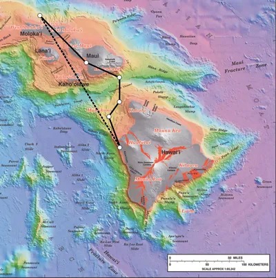
Figure 3.7 Displacement can be determined graphically using a scale map, such as this one of the Hawaiian Islands. A journey from Hawai’i to Moloka’i has a number of legs, or journey segments. These segments can be added graphically with a ruler to determine the total two-dimensional displacement of the journey. Image from OpenStax College Physics 2e, CC-BY 4.0
Vectors in Two Dimensions
A vector is a quantity that has magnitude and direction. Displacement, velocity, acceleration, and force, for example, are all vectors. In one-dimensional, or straight-line, motion, the direction of a vector can be given simply by a plus or minus sign. In two dimensions (2-d), however, we specify the direction of a vector relative to some reference frame (i.e., coordinate system), using an arrow having length proportional to the vector’s magnitude and pointing in the direction of the vector.
Figure 3.8 shows such a graphical representation of a vector, using as an example the total displacement for the person walking in a city considered in Kinematics in Two Dimensions: An Introduction. We shall use the notation that a boldface symbol, such as [latex]\text{D}[/latex], stands for a vector. Its magnitude is represented by the symbol in italics, [latex]D[/latex], and its direction by [latex]\theta[/latex].
Vectors in this Text
In this text, we will represent a vector with a boldface variable. For example, we will represent the quantity force with the vector [latex]\text{F}[/latex], which has both magnitude and direction. The magnitude of the vector will be represented by a variable in italics, such as [latex]F[/latex], and the direction of the variable will be given by an angle [latex]\theta[/latex].
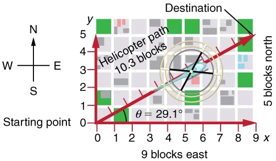
Figure 3.8 A person walks 9 blocks east and 5 blocks north. The displacement is 10.3 blocks at an angle [latex]\text{29} .\text{1}º[/latex] north of east. Image from OpenStax College Physics 2e, CC-BY 4.0
Image Description
The image shows a grid map with streets in a city layout. The map is overlaid with arrows, a compass, and labels to illustrate a path taken by a helicopter.
Below is a detailed description of the image elements:
– Compass Rose: Located on the left side of the image, it indicates north, south, east, and west directions with arrows pointing in each cardinal direction. The starting point is marked directly south.
– Grid Map: The grid is marked with blocks and numbered axes. The x-axis runs horizontally at the bottom, labeled from 0 to 9, with the direction indicated as “9 blocks east.” The y-axis runs vertically on the left, labeled from 0 to 5, with the direction marked as “5 blocks north.”
– Path and Arrows:
– A thick red arrow extends diagonally from the bottom left to the top right, representing the helicopter’s path. The path is labeled “Helicopter path 10.3 blocks” along the arrow.
– Another label near the beginning of the red arrow indicates an angle, “θ = 29.1°,” marking the angle of the path relative to the eastward direction.
– Spaced along the path are several smaller, parallel red arrows marking the intended direction of travel.
– Destination and Starting Point:
– The path begins at the “Starting point” at the bottom left (0,0) and extends to the “Destination” in the top right.
– City Blocks: The gray grid represents city blocks with random green squares, which could represent parks or important landmarks scattered throughout.
This map visualizes a helicopter’s flight path over a city grid, indicating its intended travel direction, distance, and angle from the starting point to the destination.
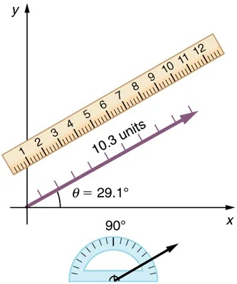
Figure 3.9 To describe the resultant vector for the person walking in a city considered in graphically, draw an arrow to represent the total displacement vector [latex]\text{D}[/latex]. Using a protractor, draw a line at an angle [latex]\theta[/latex] relative to the east-west axis. The length [latex]D[/latex] of the arrow is proportional to the vector’s magnitude and is measured along the line with a ruler. In this example, the magnitude [latex]D[/latex] of the vector is 10.3 units, and the direction [latex]\theta[/latex] is [latex]29.1º[/latex] north of east. Image from OpenStax College Physics 2e, CC-BY 4.0
Image Description
The image features a visual representation of a vector on a coordinate plane. Here’s a detailed description:
– Coordinate Axes:
– Includes a vertical y-axis and a horizontal x-axis.
– The axes intersect at the origin point (0,0).
– Ruler:
– Placed diagonally aligning from point (1,1) going upwards towards positive y and x directions.
– The ruler measures 12 units and helps illustrate another vector beneath it.
– Vector:
– A line represents the vector, drawn from the origin in a diagonal direction towards the upper right, mirroring the direction of the ruler.
– Marked with an arrowhead pointing toward the x-axis, along the line.
– The vector is labeled as 10.3 units long.
– Angle:
– The vector creates an angle of 29.1 degrees (θ = 29.1°) with the positive x-axis.
– A small arc near the origin highlights this angle.
– Protractor:
– Located below the coordinate axes to measure the angle.
– The protractor has a marked arrow pointing towards the direction of the vector, aligned with the angle measurement.
This image is likely used to demonstrate vector measurement, angle calculation, and the relationship between angles and coordinate positions.
Vector Addition: Head-to-Tail Method
The head-to-tail method is a graphical way to add vectors, described in Figure 3.10 below and in the steps following. The tail of the vector is the starting point of the vector, and the head (or tip) of a vector is the final, pointed end of the arrow.
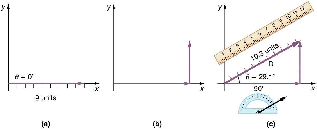
Figure 3.10 Head-to-Tail Method: The head-to-tail method of graphically adding vectors is illustrated for the two displacements of the person walking in a city considered in . (a) Draw a vector representing the displacement to the east. (b) Draw a vector representing the displacement to the north. The tail of this vector should originate from the head of the first, east-pointing vector. (c) Draw a line from the tail of the east-pointing vector to the head of the north-pointing vector to form the sum or resultant vector [latex]\text{D}[/latex]. The length of the arrow [latex]\text{D}[/latex] is proportional to the vector’s magnitude and is measured to be 10.3 units . Its direction, described as the angle with respect to the east (or horizontal axis) [latex]\theta[/latex] is measured with a protractor to be [latex]\text{29} . 1º[/latex]. Image from OpenStax College Physics 2e, CC-BY 4.0
Image Description
The image is composed of three separate panels labeled (a), (b), and (c), each showing a coordinate system with an x-axis and y-axis.
– Panel (a):
– Displays a vector along the x-axis.
– The vector is horizontal, moving right with an angle θ = 0°.
– The length of the vector is labeled as 9 units.
– Panel (b):
– Shows two vectors forming a right angle.
– One vector is horizontal along the x-axis pointing right.
– The other vector is vertical along the y-axis pointing upwards.
– Panel (c):
– Features a vector forming a triangle with the horizontal x-axis.
– The vector is diagonal, labeled as 10.3 units in length.
– The angle between the vector and the x-axis is θ = 29.1°.
– The triangle has a right angle, with the 90° highlighted.
– There is a protractor above the triangle for angle measurement and a ruler along the vector.
Each panel illustrates different properties and orientations of vectors using coordinate systems.
Step 1. Draw an arrow to represent the first vector (9 blocks to the east) using a ruler and protractor.
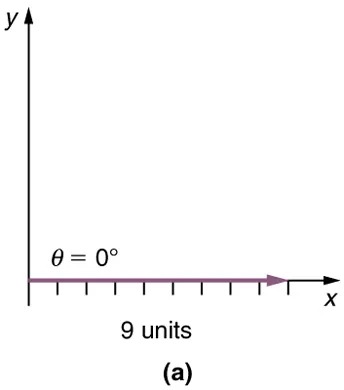
Figure 3.11 Image from OpenStax College Physics 2e, CC-BY 4.0
Image Description
The image is a coordinate plane with an x-axis and y-axis. There is a horizontal arrow along the x-axis pointing to the right, representing a vector. The vector is labeled as “9 units” in length and has an angle θ equal to 0 degrees with respect to the x-axis. The point where the vector starts is at the origin of the coordinate plane. Below the vector’s label, it is marked as “(a)”.
Step 2. Now draw an arrow to represent the second vector (5 blocks to the north). Place the tail of the second vector at the head of the first vector.
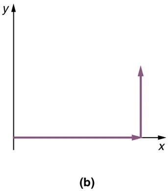
Figure 3.12 Image from OpenStax College Physics 2e, CC-BY 4.0
Image Description
The image shows a 2D coordinate system with two axes labeled “x” and “y”. The “x” axis runs horizontally from left to right, and the “y” axis runs vertically from bottom to top. Both axes are illustrated with arrows to indicate positive directions. There is a purple vector starting at the origin (0,0) extending first horizontally right along the “x” axis, then turning vertically upwards along the “y” axis. The vector forms a right angle, resembling an “L” shape, moving initially in the positive x direction and then in the positive y direction. Below the graph, there is a label “(b)”.
Step 3. If there are more than two vectors, continue this process for each vector to be added. Note that in our example, we have only two vectors, so we have finished placing arrows tip to tail.
Step 4. Draw an arrow from the tail of the first vector to the head of the last vector. This is the resultant, or the sum, of the other vectors.
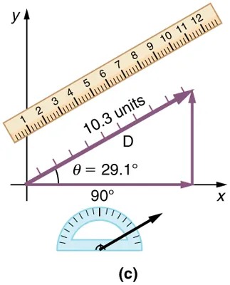
Figure 3.13 Image from OpenStax College Physics 2e, CC-BY 4.0
Image Description
The image shows a diagram with coordinate axes and a geometric representation of a vector. The x-axis is horizontal and extends to the right, while the y-axis is vertical and extends upward. A vector labeled D is drawn diagonally from the origin at an angle, with a magnitude of 10.3 units. The angle between vector D and the x-axis is indicated as 29.1 degrees.
A protractor is positioned below vector D, measuring the angle from the horizontal axis. The protractor also shows a 90-degree angle marked between the x– and y-axes. Additionally, a ruler is placed parallel to vector D, showing measurement markings from 0 to 12. The vector extends from the origin, implying a scale relevant to the ruler’s markings.
Step 5. To get the magnitude of the resultant, measure its length with a ruler. (Note that in most calculations, we will use the Pythagorean theorem to determine this length.)
Step 6. To get the direction of the resultant, measure the angle it makes with the reference frame using a protractor. (Note that in most calculations, we will use trigonometric relationships to determine this angle.)
The graphical addition of vectors is limited in accuracy only by the precision with which the drawings can be made and the precision of the measuring tools. It is valid for any number of vectors.
Example 3.1
Adding Vectors Graphically Using the Head-to-Tail Method: A Woman Takes a Walk
Use the graphical technique for adding vectors to find the total displacement of a person who walks the following three paths (displacements) on a flat field. First, she walks 25.0 m in a direction [latex]\text{49}.\text{0}º[/latex] north of east. Then, she walks 23.0 m heading [latex]\text{15}.\text{0}º[/latex] north of east. Finally, she turns and walks 32.0 m in a direction 68.0° south of east.
Strategy
Represent each displacement vector graphically with an arrow, labeling the first [latex]\text{A}[/latex], the second [latex]\text{B}[/latex], and the third [latex]\text{C}[/latex], making the lengths proportional to the distance and the directions as specified relative to an east-west line. The head-to-tail method outlined above will give a way to determine the magnitude and direction of the resultant displacement, denoted [latex]\textbf{R}[/latex].
Solution
(1) Draw the three displacement vectors.
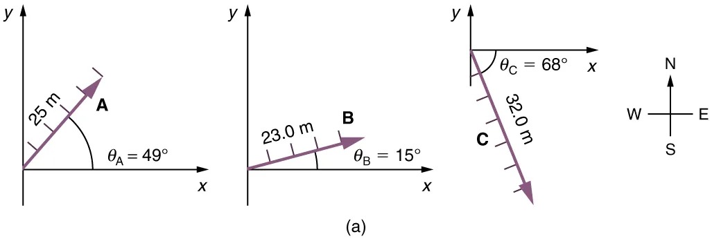
Figure 3.14 Image from OpenStax College Physics 2e, CC-BY 4.0
Image Description
The image consists of three vector diagrams labeled A, B, and C, along with a compass rose on the right. Each vector is positioned in a coordinate system with x and y axes.
– Vector A:
– The vector has a magnitude of 25 meters.
– It is oriented at an angle of 49 degrees above the positive x-axis.
– Vector B:
– The vector has a magnitude of 23 meters.
– It is oriented at an angle of 15 degrees above the positive x-axis.
– Vector C:
– The vector has a magnitude of 32 meters.
– It is oriented at an angle of 68 degrees below the negative y-axis, parallel to the negative x-axis.
– Compass Rose:
– The compass rose shows the cardinal directions: North (N), East (E), South (S), and West (W).
(2) Place the vectors head to tail retaining both their initial magnitude and direction.
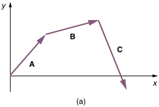
Figure 3.15 Image from OpenStax College Physics 2e, CC-BY 4.0
Image Description
The image is a graph with an x-axis labeled “x” and a y-axis labeled “y”. Three vectors labeled A, B, and C are represented by arrows forming a path breaking at two points.
– Vector A: Starts at the origin and points upward and to the right, forming an angle with the positive x-axis.
– Vector B: Begins where vector A ends, continuing upward and to the right with a smaller angle.
– Vector C: Begins at the end of vector B and points downward to the right, crossing the x-axis.
Each vector is shown with a purple arrow indicating the direction. The sequence of vectors resembles a sawtooth pattern on the graph. The label “(a)” appears at the bottom center of the image.
(3) Draw the resultant vector, [latex]\text{R}[/latex].
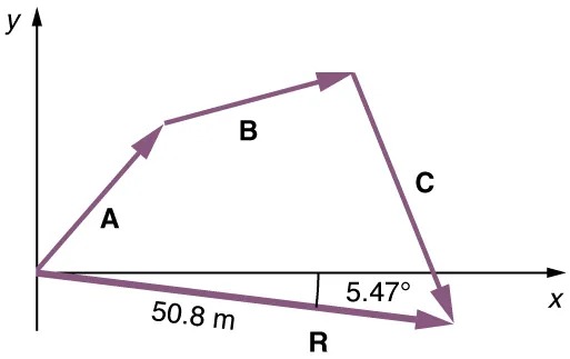
Figure 3.16 Image from OpenStax College Physics 2e, CC-BY 4.0
Image Description
The image shows a vector diagram on a coordinate plane with \(x\) and \(y\) axes. The diagram includes three vectors labeled A, B, and C, connected in a path. Each vector is depicted with an arrow indicating its direction:
– Vector A starts from the origin and points upward and slightly to the right.
– Vector B continues from the endpoint of Vector A, moving in a more horizontal direction to the right with upward ascent.
– Vector C starts from the endpoint of Vector B, heading downward with a steep angle towards the positive \(x\)-axis.
The resulting vector, labeled R, is shown pointing horizontally to the right from the origin, forming the base of the triangular path created by the vectors A, B, and C.
There are two annotations on the diagram:
– The length of the horizontal resultant vector R is marked as 50.8 meters.
– The angle between vector R and the positive \(x\)-axis is labeled as \(5.47^\circ\).
Both the x and y axes have arrows indicating positive directions, with the y-axis pointing upwards and the x-axis pointing towards the right.
(4) Use a ruler to measure the magnitude of [latex]\textbf{R}[/latex], and a protractor to measure the direction of [latex]\text{R}[/latex]. While the direction of the vector can be specified in many ways, the easiest way is to measure the angle between the vector and the nearest horizontal or vertical axis. Since the resultant vector is south of the eastward pointing axis, we flip the protractor upside down and measure the angle between the eastward axis and the vector.
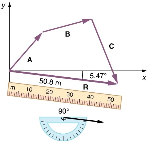
Figure 3.17 Image from OpenStax College Physics 2e, CC-BY 4.0
Image Description
The image is a diagram showing a vector addition problem and involves a coordinate system along with measurement tools.
– There is a coordinate system with an x-axis and y-axis.
– Three vectors labeled A, B, and C form a closed triangular path.
– Vector A points upward and to the left.
– Vector B points slightly downward and to the right.
– Vector C points downward and to the left.
– Each vector is represented with an arrow showing its direction and relative magnitude.
– A vector labeled R represents the resultant vector and points horizontally along the x-axis.
– The angle between vector C and the x-axis is marked as 5.47 degrees.
– A ruler below the vectors shows a measurement of 50.8 meters, positioned parallel to the x-axis.
– A protractor is shown below, indicating a 90-degree angle alignment.
The diagram visually combines geometry and measurement concepts to demonstrate how the vectors add up to form the resultant vector R.
In this case, the total displacement [latex]\textbf{R}[/latex] is seen to have a magnitude of 50.8 m and to lie in a direction [latex]5.47º[/latex] south of east. By using its magnitude and direction, this vector can be expressed as [latex]R = \text{50}.\text{8 m}[/latex] and [latex]\theta = 5 . \text{47}º[/latex] south of east.
Discussion
The head-to-tail graphical method of vector addition works for any number of vectors. It is also important to note that the resultant is independent of the order in which the vectors are added. Therefore, we could add the vectors in any order as illustrated in Figure 3.18 and we will still get the same solution.
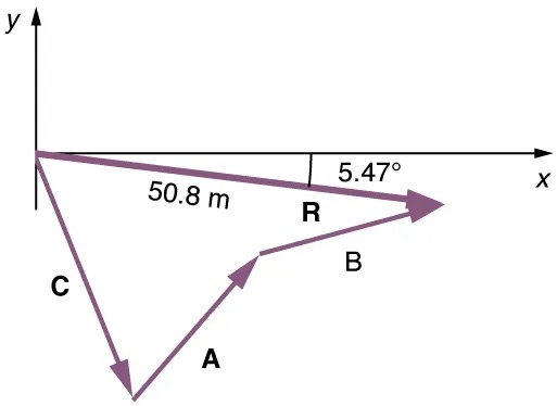
Figure 3.18 Image from OpenStax College Physics 2e, CC-BY 4.0
Image Description
The image is a diagram showing a vector addition problem on a two-dimensional Cartesian coordinate system. Here’s a detailed description of the elements:
– There are two axes: the horizontal axis labeled “x” and the vertical axis labeled “y”.
– Three vectors are labeled “A”, “B”, and “C”, each represented by arrows.
– Vector “A” points downward and slightly to the left.
– Vector “B” connects to the tip of vector “A” and points upwards and to the right.
– Vector “C” starts at the origin and points downward.
– A resultant vector, labeled “R”, is shown as the diagonal of the parallelogram formed with vectors “B” and “C”. It points approximately horizontally to the right.
– The angle between the resultant vector “R” and the positive x-axis is labeled as “5.47°”.
– The magnitude of the resultant vector “R” is labeled as “50.8 m”.
Here, we see that when the same vectors are added in a different order, the result is the same. This characteristic is true in every case and is an important characteristic of vectors. Vector addition is commutative. Vectors can be added in any order.
[latex]\textbf{A} + \textbf{B} = \textbf{B} + \textbf{A} .[/latex]
(This is true for the addition of ordinary numbers as well—you get the same result whether you add [latex]\textbf{2} + \textbf{3}[/latex] or [latex]\textbf{3} + \textbf{2}[/latex], for example).
Vector Subtraction
Vector subtraction is a straightforward extension of vector addition. To define subtraction (say we want to subtract [latex]\textbf{B}[/latex] from [latex]\textbf{A}[/latex], written [latex]\textbf{A} – \textbf{B}[/latex], we must first define what we mean by subtraction. The negative of a vector [latex]\textbf{B}[/latex] is defined to be [latex]–\textbf{B}[/latex]; that is, graphically the negative of any vector has the same magnitude but the opposite direction, as shown in Figure 3.19. In other words, [latex]\textbf{B}[/latex] has the same length as [latex]–\textbf{B}[/latex], but points in the opposite direction. Essentially, we just flip the vector so it points in the opposite direction.
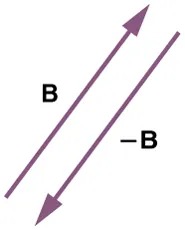
Figure 3.19 The negative of a vector is just another vector of the same magnitude but pointing in the opposite direction. So [latex]\textbf{B}[/latex] is the negative of [latex]–\textbf{B}[/latex]; it has the same length but opposite direction. Image from OpenStax College Physics 2e, CC-BY 4.0
Image Description
The image shows two diagonal arrows, each pointing in opposite directions. The arrows are parallel to each other. The arrow on the left points upward to the right, labeled “B.” The arrow on the right points downward to the left, labeled “-B.” Both arrows are colored purple. The label “B” represents the magnetic field direction, while “-B” represents the opposite direction of the magnetic field.
The subtraction of vector [latex]\textbf{B}[/latex] from vector [latex]\textbf{A}[/latex] is then simply defined to be the addition of [latex]–\textbf{B}[/latex] to [latex]\textbf{A}[/latex]. Note that vector subtraction is the addition of a negative vector. The order of subtraction does not affect the results.
[latex]\text{A}\textrm{ }–\textrm{ }\text{B}\textrm{ }=\textrm{ }\text{A}\textrm{ }+\textrm{ } \left(\right. –\text{B} \left.\right) .[/latex]
This is analogous to the subtraction of scalars (where, for example, [latex]\text{5}\textrm{ }–\textrm{ }\text{2}\textrm{ }=\textrm{ }\text{5}\textrm{ }+\textrm{ } \left(\right. –\text{2} \left.\right)[/latex]). Again, the result is independent of the order in which the subtraction is made. When vectors are subtracted graphically, the techniques outlined above are used, as the following example illustrates.
Example 3.2
Subtracting Vectors Graphically: A Woman Sailing a Boat
A woman sailing a boat at night is following directions to a dock. The instructions read to first sail 27.5 m in a direction [latex]\text{66}.\text{0}º[/latex] north of east from her current location, and then travel 30.0 m in a direction [latex]\text{112}º[/latex] north of east (or [latex]\text{22}.\text{0}º[/latex] west of north). If the woman makes a mistake and travels in the opposite direction for the second leg of the trip, where will she end up? Compare this location with the location of the dock.
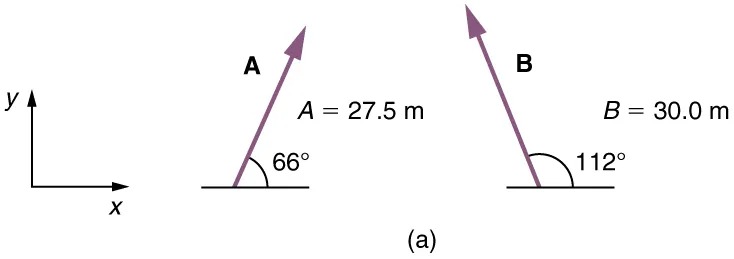
Figure 3.20 Image from OpenStax College Physics 2e, CC-BY 4.0
Image Description
The image consists of two vectors labeled A and B, shown in a two-dimensional plane with coordinate axes.
– Vector A:
– Magnitude: 27.5 meters
– Direction: The arrow is directed upwards and to the right, forming an angle of 66 degrees with the horizontal axis.
– Vector B:
– Magnitude: 30.0 meters
– Direction: The arrow is directed upwards and to the left, forming an angle of 112 degrees with the horizontal axis.
– The coordinate axes are labeled with x (horizontal) and y (vertical) directions. The arrows representing the vectors are colored and have arrows at one end to indicate direction.
Strategy
We can represent the first leg of the trip with a vector [latex]\textbf{A}[/latex], and the second leg of the trip with a vector [latex]\textbf{B}[/latex]. The dock is located at a location [latex]\textbf{A } + \textbf{ B}[/latex]. If the woman mistakenly travels in the opposite direction for the second leg of the journey, she will travel a distance [latex]B[/latex] (30.0 m) in the direction [latex]180º – 112º = 68º[/latex] south of east. We represent this as [latex]–\textbf{B}[/latex], as shown below. The vector [latex]–\textbf{B}[/latex] has the same magnitude as [latex]\textbf{B}[/latex] but is in the opposite direction. Thus, she will end up at a location [latex]\textbf{A} + \left(\right. –\textbf{B} \left.\right)[/latex], or [latex]\textbf{A} – \textbf{B}[/latex].
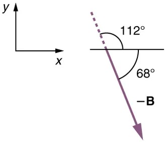
Figure 3.21 Image from OpenStax College Physics 2e, CC-BY 4.0
Image Description
The image shows a two-dimensional coordinate system with x and y axes. A vector labeled “-B” is positioned in the plane. The vector is angled downward to the right, creating a 68-degree angle with the positive x-axis. There is an additional angle labeled 112 degrees between a dashed line extending the vector backward and the positive x-axis. The vector arrow is depicted as pointing in the downward direction to the right.
We will perform vector addition to compare the location of the dock, [latex]\text{A}\textrm{ } +\textrm{ } \mathbf{B}[/latex], with the location at which the woman mistakenly arrives, [latex]\text{A}\textrm{ }+\textrm{ } \left(\right. –\text{B} \left.\right)[/latex].
Solution
(1) To determine the location at which the woman arrives by accident, draw vectors [latex]\textbf{A}[/latex] and [latex]–\textbf{B}[/latex].
(2) Place the vectors head to tail.
(3) Draw the resultant vector [latex]\mathbf{R}[/latex].
(4) Use a ruler and protractor to measure the magnitude and direction of [latex]\mathbf{R}[/latex].
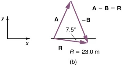
Figure 3.22 Image from OpenStax College Physics 2e, CC-BY 4.0
Image Description
The image contains two main components:
- A set of axes on the left, labeled x and y, representing a Cartesian coordinate system.
- A vector diagram on the right. This diagram consists of three vectors that form a triangle. The vectors are labeled as A, -B, and R.
- Vector A is pointing upwards to the right.
- Vector -B is pointing downwards to the left and forms a 7.5-degree angle with the horizontal line extended from R.
- Vector R is pointing horizontally to the right and is labeled as R = 23.0 m.
The equation A – B = R is written above the triangle diagram.
In this case, [latex]R = \text{23} . \text{0 m}[/latex] and [latex]\theta = 7 . \text{5}º[/latex] south of east.
(5) To determine the location of the dock, we repeat this method to add vectors [latex]\textbf{A}[/latex] and [latex]\textbf{B}[/latex]. We obtain the resultant vector [latex]\textbf{R} '[/latex]:
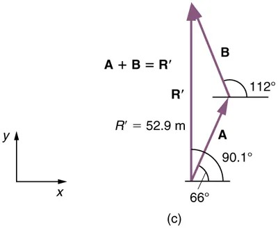
Figure 3.23 Image from OpenStax College Physics 2e, CC-BY 4.0
Image Description
The image illustrates a vector addition diagram on a two-dimensional plane with an x-y axis. There are two vectors, labeled A and B, which are being added to form a resultant vector R’. Here’s a detailed description:
- The x-y axis is shown on the left side of the image, with arrows indicating the positive x-direction pointing to the right and the positive y-direction pointing upwards.
- Vector A is drawn starting at a horizontal line, making an angle of 66 degrees with the x-axis. Its angle relative to the horizontal is marked as 90.1 degrees. It points upwards and to the left.
- Vector B is drawn starting from the tip of vector A, making an angle of 112 degrees with the resultant vector R’. It points upwards and to the right.
- The resultant vector R’ is drawn vertically upwards from the starting point of vector A. The magnitude of R’ is labeled as 52.9 meters.
- The equation A + B = R’ is written beside the vectors, indicating that the vectors A and B are added to produce the resultant vector R’.
In this case [latex]R \textrm{ }=\textrm{ }\text{52}.\text{9 m}[/latex] and [latex]\theta = \text{90}.\text{1}º[/latex] north of east.
We can see that the woman will end up a significant distance from the dock if she travels in the opposite direction for the second leg of the trip.
Discussion
Because subtraction of a vector is the same as addition of a vector with the opposite direction, the graphical method of subtracting vectors works the same as for addition.
Multiplication of Vectors and Scalars
If we decided to walk three times as far on the first leg of the trip considered in the preceding example, then we would walk [latex]\text{3}\textrm{ } \times \textrm{ }\text{27} . \text{5 m}[/latex], or 82.5 m, in a direction [latex]\text{66} . 0 º[/latex] north of east. This is an example of multiplying a vector by a positive scalar. Notice that the magnitude changes, but the direction stays the same.
If the scalar is negative, then multiplying a vector by it changes the vector’s magnitude and gives the new vector the opposite direction. For example, if you multiply by –2, the magnitude doubles but the direction changes. We can summarize these rules in the following way: When vector [latex]\mathbf{A}[/latex] is multiplied by a scalar [latex]c[/latex],
- the magnitude of the vector becomes the absolute value of [latex]c[/latex][latex]A[/latex],
- if [latex]c[/latex] is positive, the direction of the vector does not change,
- if [latex]c[/latex] is negative, the direction is reversed.
In our case, [latex]c = 3[/latex] and [latex]A = 27.5 m[/latex]. Vectors are multiplied by scalars in many situations. Note that division is the inverse of multiplication. For example, dividing by 2 is the same as multiplying by the value (1/2). The rules for multiplication of vectors by scalars are the same for division; simply treat the divisor as a scalar between 0 and 1.
Resolving a Vector into Components
In the examples above, we have been adding vectors to determine the resultant vector. In many cases, however, we will need to do the opposite. We will need to take a single vector and find what other vectors added together produce it. In most cases, this involves determining the perpendicular components of a single vector, for example the x– and y-components, or the north-south and east-west components.
For example, we may know that the total displacement of a person walking in a city is 10.3 blocks in a direction [latex]\text{29} .\text{0}º[/latex] north of east and want to find out how many blocks east and north had to be walked. This method is called finding the components (or parts) of the displacement in the east and north directions, and it is the inverse of the process followed to find the total displacement. It is one example of finding the components of a vector. There are many applications in physics where this is a useful thing to do. We will see this soon in 3.4 Projectile Motion, and much more when we cover forces in Dynamics: Newton’s Laws of Motion. Most of these involve finding components along perpendicular axes (such as north and east), so that right triangles are involved. The analytical techniques presented in Vector Addition and Subtraction: Analytical Methods are ideal for finding vector components.
PhET Explorations
Maze Game
Learn about position, velocity, and acceleration in the “Arena of Pain”. Use the green arrow to move the ball. Add more walls to the arena to make the game more difficult. Try to make a goal as fast as you can.
