Neurophysiology Lab Outline
Introduction
The Nervous System and Neurons
Everything that we sense in the world, and all of the movements that we perform, are due to activity in the nervous system. The afferent branch of your (human) peripheral nervous system (PNS) - the sensory nervous system - sends information about touch, sound, sight, smell, and taste towards your central nervous system (CNS, brain and spinal cord). The efferent branch of your PNS – the motor system – sends motor commands to your muscles, in response to sensory input. If you would like to review the nervous system in more detail (i.e. structure, function, action potentials and communication between neurons) check out this resource.
Neurons are the basic unit of the nervous system. Most neurons have a small anatomical gap between them called a synapse, and neurons typically release chemicals that diffuse across the synapse to affect other neurons. (Note the qualifiers “most” and “typical.” Neurons are very diverse in their anatomy and physiology, and this description can only discuss common features of neurons.)
How a nervous system functions depends in large part on the physiological connections between the neurons. The connections are often described as a “circuit” by analogy with electrical circuits, although neural circuits differ in important ways. For example, connections between neurons are much more dynamic and flexible than in electrical circuits. Be suspicious if you hear someone saying brains are “hard-wired” for things!
Models of the Nervous System
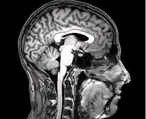
We are limited to some lower resolution imaging techniques if we want to look at living human brains - such as magnetic resonance imaging (MRI), or computerized tomography (CT) scans. If we want to look deeper, at the actual neurons, this requires tissue that has been removed from an organism. While a muscle biopsy or tumour biopsy might be something you see in human medicine for histological purposes, you definitely would not be taking an entire coronal section of a human brain unless this came from an individual who had passed away and donated their body to science, or if an autopsy was being performed.
We can, however, work with model organisms. Just like in the histology lab, tissues can be collected from a model organism for research studies. The use of model organisms requires extensive ethical consideration, and in order to use and euthanize mice for a research study, your proposal must be examined and approved by the Canadian Council for Animal Care (CCAC) and your institutional animal ethics board (at McMaster, this is called the McMaster Animal Research Ethics Board (AREB)).
Brain models are important for researchers to learn more about neurodegenerative diseases, such as Alzheimers, Parkinson's, Huntington's, or Amyotrophic Lateral Sclerosis (ALS). It is difficult to see just how the neurons are being affected by a neurodegenerative disease in a clinical setting, and the use of a model organism allows us to look more closely and extrapolate those findings back to other mammals. One model for neuroinflammation in a mouse model is to induce a stroke in the brain through the blocking off of a major arterial blood supply temporarily, a procedure adapted by Moisse et al. (2008) when generating the tissue slides we will be working with today. This is called middle cerebral artery occlusion (MCAo), which is performed surgically and temporarily (30 minute duration) in live animals. Animals are anesthetized using a small mask during the surgery, and neurobehavioural assessments are performed during the occlusion (while the artery is blocked off), as well as immediately following reperfusion (after the blockage has been removed and blood re-enters this region of the brain) and 24 and 72 hours post-reperfusion. After the surgery, the mice receive antibiotics and analgesics, as well as a special nutritional supplement and extra fluids as required (subcutaneously injected, like when a human gets an IV bag at the hospital).
The resulting neuroinflammatory response in the brain tissues of these mice after the induced stroke varies by individual, but common damage includes necrotic lesions in the cortex and subcortex, as well as lesions in the motor cortex of the hemisphere of the brain that experienced the stroke. It is suspected that the lesions are caused by microglial activation, which triggers a protective response when the neurons are damaged. Importantly, this MCAo procedure induces a stroke in just one hemisphere of the mouse brain, which allows the researcher to consider the two hemispheres of the mouse as paired data (one side of the brain can be considered a control group data point, and the other a treatment group data point).
The slides we will be working with today come from the doctoral research of Dr. Katie Moisse, a Life Sciences Program professor. The mouse brains have been sectioned into 5μm thick coronal sections (recall back to the different anatomical planes) and stained with an H&E staining protocol (which you will get to perform during the histology staining lab!). These mice received the MCAo intervention described above, and the slide you will work with contains two slices of brain (not every slide is from the same region of the brain, some are more anterior and some more posterior) as well as eight slices of spinal cord. We will be using the brain sections today, but the spinal cord sections are there for if you are interested in exploring what those pieces of tissue look like at the end of the session.
Safety Precautions
These slides have been donated to us, and are fragile and in low supply (i.e. if you break them, there are no more slides and this lab won't be continued in future offerings of LIFESCI 2L03). Please use extreme care when handling these specimens.
- The slides are already placed on the microscope. At no point during this lab will you be required to remove the slide from the microscope, you can leave it on the stage.
- The stage micrometer image has been prepared for you, and can be found on the lab computer desktop.
Lab Overview and Timeline
| Time (min) |
What will you be doing? | Total Time (min) |
|---|---|---|
| 0 - 10 | Overview of lab activities by the TA. Fill in the pre-lab if you have not completed yet. | 10 |
| 10 - 120 | Lab Part 1: Landmarking, Image Capture, and ImageJ Analysis Lab Protocol 1: Using Anatomical features to identify anterior/posterior position of your coronal brain tissue section Lab Protocol 2: Capturing Images from Brain Samples for Measurements Lab Protocol 3: Measuring the lesion area and lesion density in each hemisphere |
110 |
| 120 - 170 | Lab Part 2: Statistical Analysis of the Class Data Set Lab Protocol 4: Running your Statistical Tests Submit your ELN at the end of lab. |
50 |
In this lab, you will be investigating coronal sections of mouse brains for lesions around the neurons that are indicative of neurodegeneration as a result of an induced stroke in one hemisphere of the brain. You will also examine the tissue sections for necrotic regions of tissue, which may also occur in some mice as a result of occlusion of blood flow during the performed surgery. You will then gather data in pairs, and perform a statistical analysis (a t test) to determine if the findings are significant. These results will be reported as part of your DLR 2 assignment.
Lab Part 1: Landmarking, Image Capture, and ImageJ Analysis
Purpose
To estimate where approximately in the brain this tissue section was obtained from (anterior/posterior). To measure the quantity of lesions per mm2 in each hemisphere of each of the two brain sections at your station, and to measure the average size of a lesion in each hemisphere of each of the two brain sections.
Summary of Activities
Follow protocol 1 to locate the approximate position of the tissue section in the whole mouse brain using an online atlas. Follow protocol 2 and protocol 3 to complete the measurements required for the class dataset.
When the stroke was induced in this mouse, via the occluded blood vessel (recall, the middle cerebral artery occlusion, abbreviated to MCAo), the blood flow was cut off to one side of the brain for 30 minutes. The hypothesis (and prediction) we are working with today is:
IF MCAo results in neurodegeneration/tissue damage to the brain (in the form of necrotic infarcts (big, dead deteriorated regions of tissue) and lesions around the neuron cell bodies (hollow spaces around cell bodies that are viewable because the tissue has been stained with H&E), THEN the side of the mouse brain that experienced the loss of blood flow will exhibit more neurodegeneration/tissue damage relative to the other hemisphere.
You will be working together in pairs (group of 2) to create a data set. There are only 6 mouse brain slides available for the class to use, where each pod will receive one slide. The slide you'll be working with is already located at your station on the microscope stage, to minimize risk of slips/drops of these very irreplaceable slides. Each pair in your pod will capture images from one of the two brain sections (referred to as Mouse 1 and Mouse 2) and measuring the size of 5 lesions in each hemisphere in 3 regions of interest (ROI). Your group will generate 30 values total for lesion area. You will also calculate the number of lesions per mm2 in each hemisphere (6 values total calculated per pair of students). These measurements will be calculated by capturing images and using the area measurement tool in ImageJ. You will also be capturing an image of the brain at 40x magnification for the purpose of labeling parts of the mouse brain using the Brain Anatomy Atlas as a guide.
Materials
- Prepared H&E stained mouse brain tissue slide (use extreme caution when handling these specimens)
- Stage Micrometer image located on computer desktop
- Zeiss Primostar 3 microscope and microscope camera
- Zen software
- ImageJ software
- Brain Anatomy Atlas
- Table Templates (download a copy and fill in at your group's station)
Lab Protocol 1: Using Anatomical features to identify anterior/posterior position of your coronal brain tissue section
- Navigate to the Brain Anatomy Atlas website. Select the "Coronal Atlas" option to view all of the sections in a file folder view, or launch the interactive atlas viewer for the [coronal] option to jump into the interactive slider format.
- each of these atlas images has been coloured in with labels on one side of the image. Selecting that image will let you identify what zone the colours represent (such as blue, which represents the cerebrum, or red, which represents the brainstem), but the information on the left legend can be expanded to define each of the acronyms labelling specific structures in the zones as well.
- the other half of the image in the atlas looks more like the tissue you are viewing under the microscope. It has been stained using a slightly different protocol, so the colours do not match perfectly to the colours you will see on your slide. (Specifically, the pink eosin counterstaining is not present in the atlas images to provide contrast and make it clear where there is empty space).
- The tissue slices in the atlas are numbered. "Position 1" is located at the most anterior part of the mouse brain - these two lobes are related to the mouse's sense of smell, and are called olfactory bulbs. "Position 527" is the most posterior part of the mouse brain, and is the analogous structure to our medulla (coloured in pink). Just slightly anterior from here, you'll find the cerebellum (coloured in yellow).
- Set up your microscope by placing it in Kohler alignment and focusing on your microscope slide at a low objective (4X objective). If you do not remember how to set up your microscope, refer to Appendix E - Microscopes. Pan around the view of your brain tissue using the x and y knobs. Try to get a sense of the approximate shape of the brain tissue present on your slide. (Some of you may see some holes in the middle of your brain section - these are the ventricles, which will be a very good hint as to where spatially your section came from! Others may see very clear outer perimeter shapes, or perhaps the hippocampus, which looks like a dragonfly, which can help you to landmark if you are towards the anterior or posterior of the brain.) NOTE: Some of the slides may have a yellow background appearing in Zen rather than a white background - this is an artefact from the coverslip glue on these samples. You do not need to try and remove the yellowing in your images.
- Head over to the atlas, and compare the shape of the tissue you have to the slices of the mouse brain in the atlas. Identify a slice that is approximately the same as the tissue you have on your slide and write down the approximate slice (i.e. position number) from the atlas that corresponds with your sample in your ELN. This will NOT be graded for accuracy. We want you to get a sense of WHERE in the brain you'll be looking today (i.e. front of the mouse brain (anterior) or rear of the mouse brain (posterior). The structures you see may vary depending on where your tissue section originated in the whole brain (e.g. brain stem, cerebellum, frontal lobe).
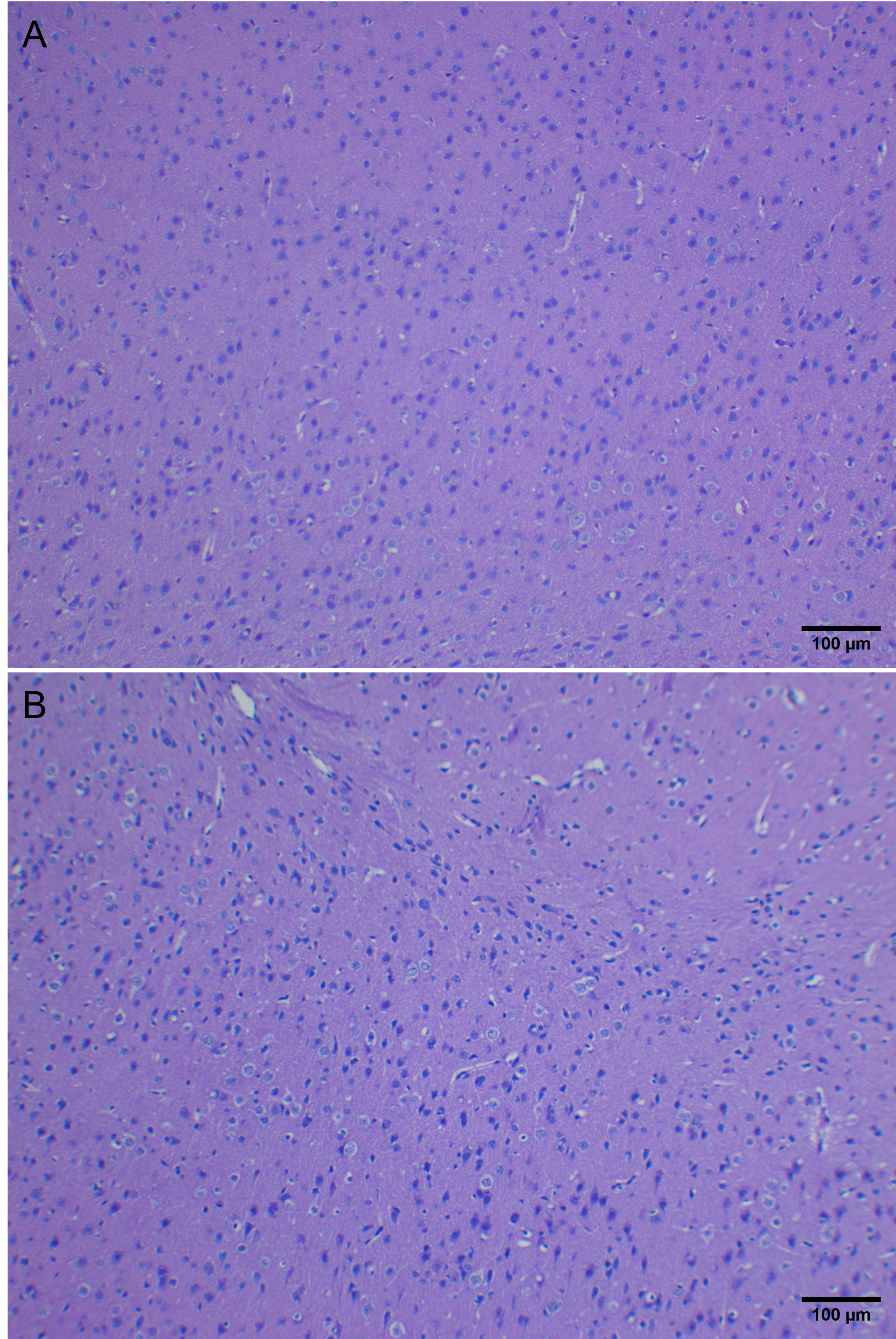
Capture an image of your mouse brain at 40x magnification (4x objective), focusing on the anterior region of the brain. We have provided an example image below. Refer to the Microscope Appendix for the Primostar microscope and the Zen Software Appendix for directions on using the microscope and software to capture and export your image. 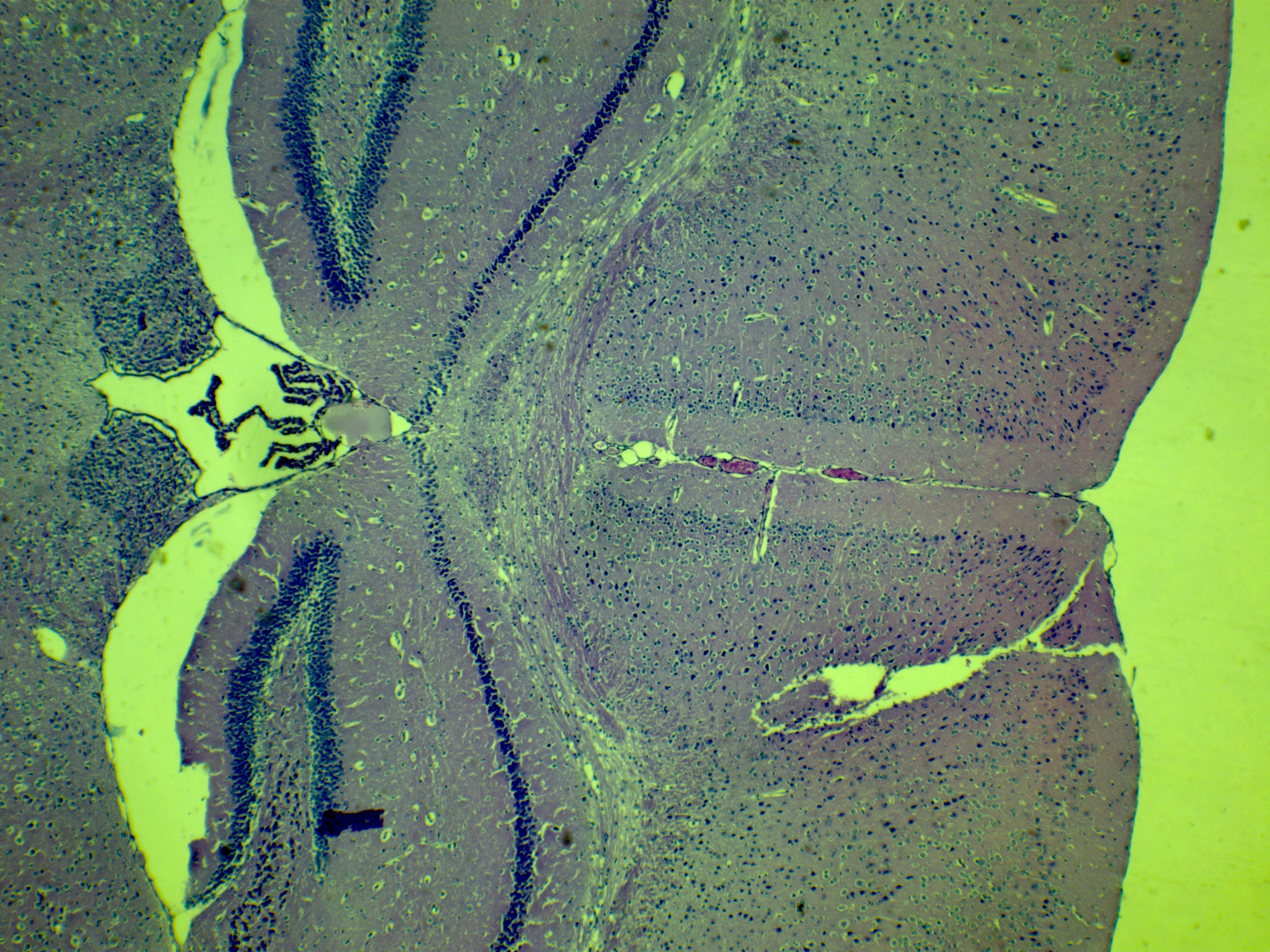 Figure 3: Example image of a coronal section of the mouse brain at 40x magnification. Image is oriented ventral to dorsal (left to right). Note: The background of this image is yellow due to slide preparation. Some of you may observe the same on your slides.
5. We are going to be counting lesions located in the cortex of the mouse brain. The cortex (CTX, a green colour in the atlas) is a part of the cerebrum, along the outer perimeter of the brain (this part is the most superficial layer). Regardless of where your section is placed in the brain, all of these slices have some cortex along the outer layer of the tissue section. Take some time to look at the atlas and familiarize yourself with where the cortex is found in your tissue layer.
Did you notice any necrotic infarcts in the brain tissue while you were exploring? This would look something like THIS:
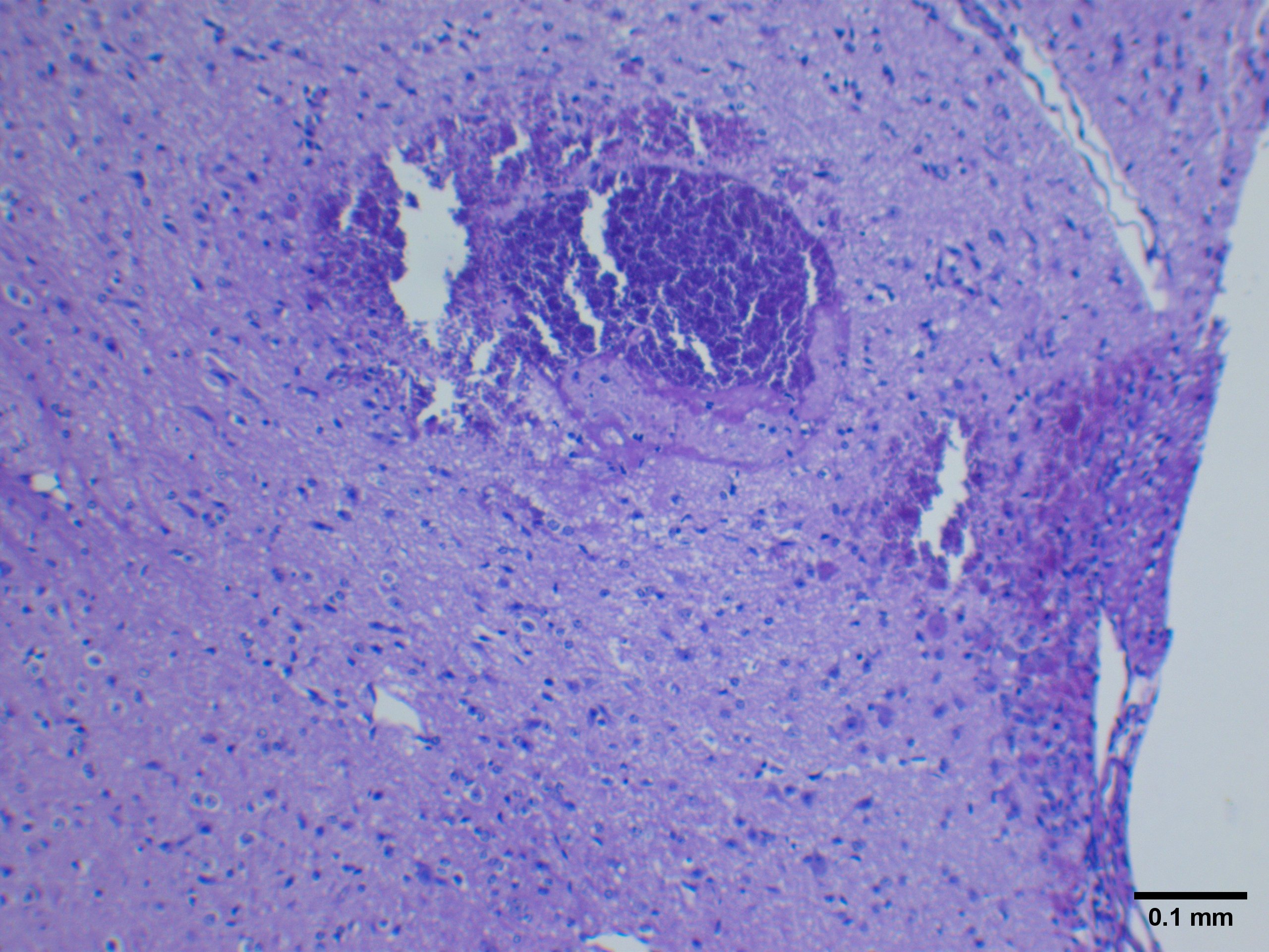
Not every slide has an example of a necrotic infarct, so we won't be quantifying any of these this week - however, if you were Dr. Moisse, you may have wanted to take the surface area of these infarcts to see how much damaged tissue was present. We will be learning about surface area measurements using ImageJ in protocol 2 and 3.
Lab Protocol 2: Capturing Images from Brain Samples for Measurements
Each microscope in the Living Systems Lab has an instructional guide located in the appendix of this Pressbook, in addition to guides for using the software required for this activity. Refer to the following relevant appendices as needed during this activity:
NOTE: Since there is only one slide per pod, one pair of students will have to wait briefly to gain access to the slide while the other group takes images. The group that is waiting may use that time to start their ELN and use the atlas to annotate their brain image from Protocol 1, as this will be expected for your DLR assignment.
- You will work together in pairs (or a group of 3 if there is an odd number of students in the class) to capture three images, or regions of interest (ROI) of the cortex from each hemisphere on your slide. (Remember, you've taught yourself where the cortex is on your tissue sample using the atlas in the last protocol). This is a total of (6) images per pair of students in the pod. One pair will take images for Mouse 1 while the other pair will take images for Mouse 2.
- 1st pair of students: Mouse 1 Brain - Side A (healthy) x3
- 1st pair of students: Mouse 1 Brain - Side B (lesioned) x3
- 2nd pair of students: Mouse 2 Brain - Side A (healthy) x3
- 2nd pair of students: Mouse 2 Brain - Side B (lesioned) x3
- Focus on the slide at a low magnification to start, and slowly work your way up to the 400X total magnification (using the 40X objective). You will capture your images at this magnification. Ensure you capture images from the cortex for all 6 images.
- Save these six images with descriptive titles, so you will be sure to remember where the image is from, the magnification, etc. on your own personal OneDrive (or equivalent).
- This week, you do not need to capture an image of the stage micrometer yourselves - these images have been prepared for you and saved to the lab computer desktop. You still require this image of the stage micrometer to calibrate ImageJ, but we do not want you to remove these microscope slides from the microscope this week, to ensure no slides are damaged. Be sure to download and save the stage micrometer image to your OneDrive.
Lab Protocol 3: Measuring the lesion area and lesion density in each hemisphere
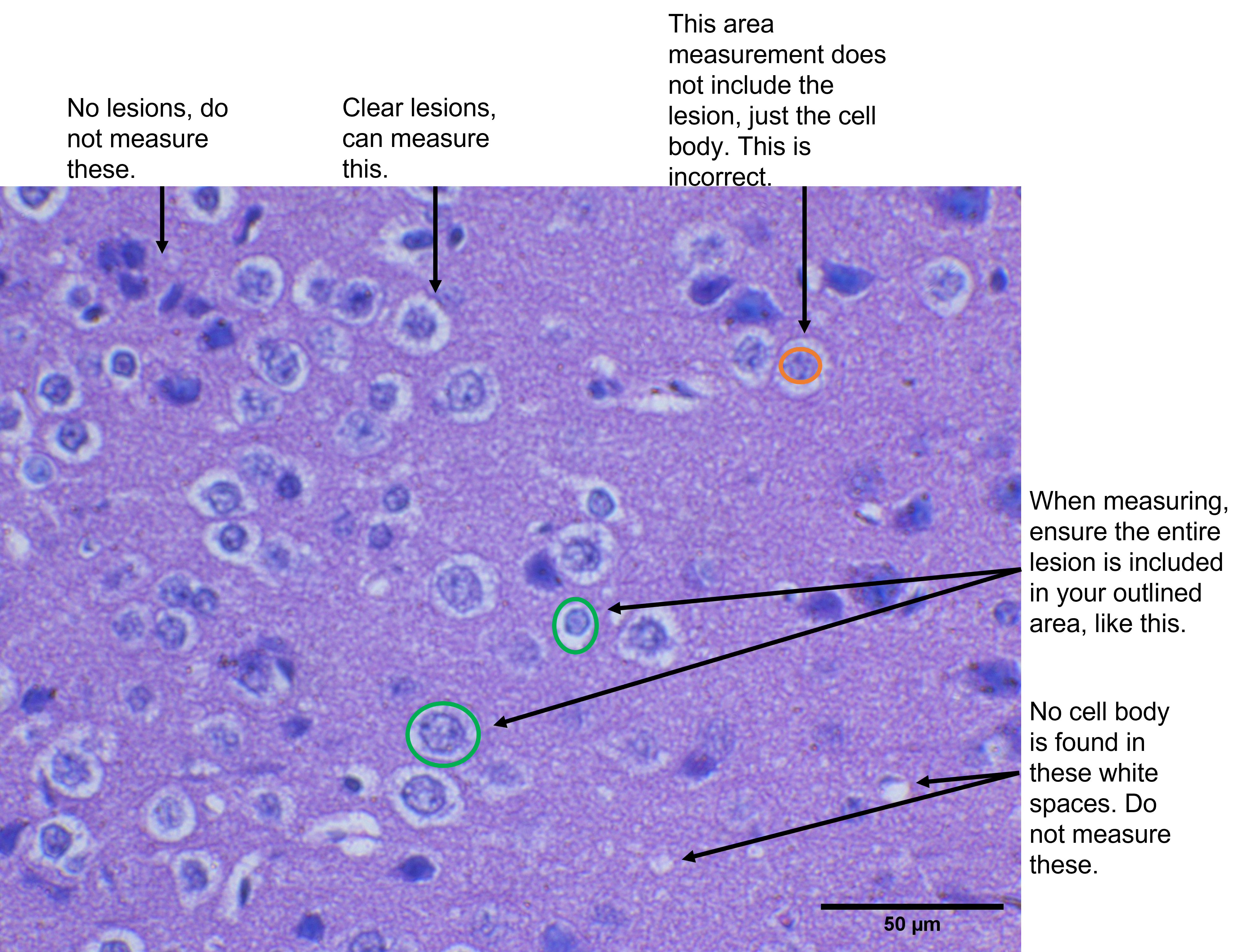
The brain lesions can be a bit challenging to spot at first. Take a look at figure 5 below, to refer to some examples of what a lesion looks like, what should be ignored, and where to make your area measurements for these lesions.
- If you have not already, download a copy of the Table Templates, and use it to record your measurements as you analyze your brain sections with ImageJ.
- Follow the steps in the ImageJ Appendix to calibrate ImageJ using your scale bar. You will also want to make sure that your results window will show you the area measurement - the ImageJ appendix also demonstrates how to ensure you have the correct measurement tools available in your results window.
- For each image, you are going to randomly select 5 lesions to take an area measurement of. You can use either the freehand or the polygon selection tool to trace the outline of the structure of which you wish to measure the area. Record the values in your template table I as you complete these measurements.
- NOTE: the values for the area of each lesion should be recorded in units of μm2
- You will have a total of 30 values recorded in your table when you have completed this part of the analysis.
- Next, you will want to take the surface area of the entire image - we are going to calculate the density of the lesions in each image, and to do so, we need to know the total surface area we will be counting lesions within. There is another selection tool shaped like a rectangle that will be helpful here.
- If the whole image contains too many lesions to count, you can also use a smaller area. Using the rectangle selection tool, you can select a smaller zone within the image and calculate the area of that zone. Then, count just the lesions within that zone.
- If a lesion is on the edge/perimeter of the image/zone, count this as a HALF lesion, rather than a whole lesion. Counting is not a perfect science - sometimes, we need to create rules that adjust how we count to ensure higher accuracy in our measurements. You will encounter another type of counting rule in a future lab when we try counting cells in a haemocytometer.
- Perform a count of how many lesions you can see in each of the six images. Record the population density of the lesions (in units of lesions/mm2) in your template table II.
- NOTE: the values for the lesion density should be recorded in units of lesions/mm2
- Upload your raw data table in your ELN as a record of your work for this week.
Lab Part 2: Statistical Analysis of Your Data
Purpose
To analyze your data and run t tests to determine if the findings are significant.
Summary of Activities
Use GraphPad to determine if your results are significant using the t test calculator. Report your results in your Crowdmark ELN. You will also need these results for your DLR assignment.
Materials
- Computer with internet access to the GraphPad calculator
- Your area of lesion and lesion density measurements that you inputted into the table templates (Tables I and II)
Lab Protocol 4: Running your Statistical Tests
- Open your table template in excel on your lab computer.
- There are two sets of recorded data to analyze, and you'll want to keep them distinct.
- ensure you have the correct sample size (N) recorded for each of your t tests. Remember for this lab, N refers to the number of data points collected for each hemisphere. These would be technical replicates, since you collected multiple measurements from the same single source (i.e. brain hemisphere).
- you should calculate the average and standard deviation. You can do this in the excel spreadsheet. You will NOT put these values into the t test calculator, however - you'll want to use the raw data values to complete the t test.
- Run your t tests using this GraphPad calculator.
- In box 1 (Choose data entry format), select 'Enter up to 50 rows' or 'Enter or paste up to 2000 rows'.
- In box 2 (Choose a test), select 'paired t test'.
- Consider: why is this data "paired" and not unpaired?
- In box 3 (Enter data), enter your data for each condition (remember, you'll do one experiment at a time for this, you cannot combine the results for the lesion density and the area of lesions) and provide an appropriate label for each category.
- In box 4 (View the results), select 'Calculate now'.
- Take a screen shot of the paired t test result for each of the two investigations (lesion density and area of lesions).
- Use the links provided on the test result screen to help you understand and interpret the t test result. These links will take you to the GraphPad Prism Statistics Guide. Some of the relevant links are:
- Report your results and paste the screenshots in your Crowdmark ELN.
Lab Exit Checklist
- Locate the approximate spatial position of the brain sections you have been assigned to work with at your pod, using the Atlas tool
- Capture one image of the brain at 40x, including a scale bar, and upload the image to Crowdmark.
- Capture six images of the brain cortex, three in each of the two hemispheres of the brain assigned to you on the microscope slide. Ensure you have clearly labeled your images so you know which is which.
- Upload your two best images at 400x (one for each hemisphere), including a scale bar, to Crowdmark.
- Calibrate ImageJ and measure the lesion density and the surface area of 5 lesions in each image. Record these values in the template tables (I and II). Upload your template tables, fully filled in, to your Crowdmark ELN.
- Run t tests on your two sets of data and upload screenshots of the results to Crowdmark.
- Submit your ELN on Crowdmark before leaving the lab.
- Save all your images for the DLR assignment to your OneDrive, as well as the stage micrometer image that was provided to you. You will also need to save your data from the table templates.
- Be sure to log out of all personal accounts before leaving the lab computer.
References
Moisse, K., Welch, I., Hill, T., Volkening, K., & Strong, M. J. (2008). Transient middle cerebral artery occlusion induces microglial priming in the lumbar spinal cord: a novel model of neuroinflammation. Journal of neuroinflammation, 5(1), 1-9. https://doi.org/10.1186/1742-2094-5-29
Images
creative commons image
