20 RStudio Workshop: Two-Way ANOVA
Within-Participants Two-Way ANOVA
We can use the same function that was used to compute a one-way within-subjects ANOVA for a two-way ANOVA. I highly encourage you to attempt to conduct the analyses on your own before progressing further into this guide.
For this exercise, we will be looking at the data file named "Practice_2WayANOVA_Within.xlsx"
- Measured Variable: TestScore
- 2 x 3 Repeated-Measures Design
- Factors: "Beverage" and "Sleep"
In this hypothetical experiment, participants attended 6 lectures across different time points. After a lecture, they were asked to sleep for 0 hours, 5 hours, or 8 hours before coming back the next day to be quizzed on the lecture content. At the time of test, they were given either coffee or a placebo (decaffeinated hot beverage).
We are interested in whether Test Scores suffer when participants don't receive enough sleep, and whether consuming coffee alleviates that performance decrement.
mydata2w <-read_excel("Practice_2WayANOVA_Within.xlsx") #importing our data file
mydata2w <- mydata2w %>%convert_as_factor(ID, Gender, Beverage, Sleep) #setting up factorsstr(mydata2w) #checking factors
## tibble [516 × 6] (S3: tbl_df/tbl/data.frame)## $ ID : Factor w/ 86 levels "29057","32239",..: 20 48 84 61 22 23 25 29 72 69 ...## $ Gender : Factor w/ 3 levels "F","M","Non-Binary": 1 2 1 1 1 1 1 2 1 1 ...## $ Age : num [1:516] 25 22 22 20 22 20 21 20 19 21 ...## $ Beverage : Factor w/ 2 levels "Coffee","Placebo": 1 1 1 1 1 1 1 1 1 1 ...## $ Sleep : Factor w/ 3 levels "0","5","8": 1 1 1 1 1 1 1 1 1 1 ...## $ TestScore: num [1:516] 99 64.3 93.3 94.8 89.1 ...
# Summary Statistics Tablemydata2w.summarystat <- mydata2w %>%group_by(Beverage, Sleep) %>%get_summary_stats(TestScore, type = "full")
# Selecting rows of data only if ID value is uniquemydata2w.unique <- mydata2w %>%distinct(mydata2w$ID, .keep_all=TRUE) # Looking at the distribution of "Gender" in our sample sizetable(mydata2w.unique$Gender)
## ## F M Non-Binary ## 60 21 5
# Mean Age of Sample Sizemydata2w.unique %>%get_summary_stats(Age, type ="mean")
## # A tibble: 1 × 3## variable n mean## <fct> <dbl> <dbl>## 1 Age 86 21.5
mydata2w.summarystat
## # A tibble: 6 × 15## Beverage Sleep variable n min max median q1 q3 iqr mad mean## <fct> <fct> <fct> <dbl> <dbl> <dbl> <dbl> <dbl> <dbl> <dbl> <dbl> <dbl>## 1 Coffee 0 TestSco… 86 51.2 99.0 96.1 90.6 97.6 7.01 4.27 91.7## 2 Coffee 5 TestSco… 86 64.3 99.0 97.6 94.8 99.0 4.22 2.09 95.7## 3 Coffee 8 TestSco… 86 64.3 99.0 97.6 94.8 99.0 4.17 2.06 96.0## 4 Placebo 0 TestSco… 86 -6.95 74.8 23.2 14.2 40.4 26.2 18.8 28.2## 5 Placebo 5 TestSco… 86 -1.67 79.1 62.2 45.1 70.0 24.8 14.8 56.4## 6 Placebo 8 TestSco… 86 30.0 79.1 71.6 64.9 74.9 10.1 6.82 67.5## # ℹ 3 more variables: sd <dbl>, se <dbl>, ci <dbl>
Visualization
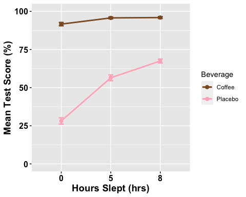
# Line plots with multiple groupsanova2w.lineplot <-ggline(mydata2w, x = "Sleep", y = "TestScore", color = "Beverage",add =c("mean_se"), #adding standard error barspalette =c("tan4", "pink1"),order =c("0", "5", "8"), #organizing order of levelsylab = "Mean Test Score (%)", xlab = "Hours Slept (hrs)", #x- and y-axis title linetype = "solid", font.label =list(size = 20, color = "black"),size = 1,ggtheme =theme_gray(),ylim=c(0,100) #adjusting the min and max value of y-aixs )
# Change the appearance of titles and labelsanova2w.lineplot +font("xlab", size = 14, color = "black", face = "bold")+font("ylab", size = 14, color = "black", face = "bold")+font("xy.text", size = 12, color = "black", face = "bold")
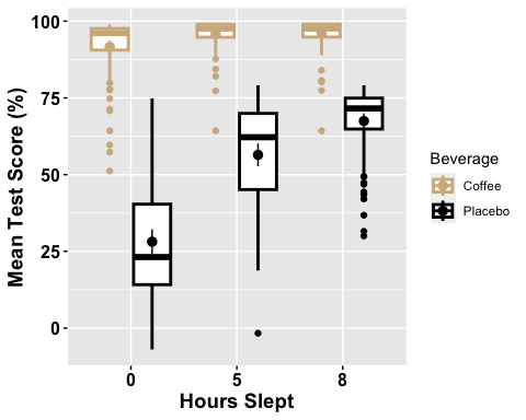
# Box plot with two factor variablesanova2w.boxplot <-ggboxplot(mydata2w, x = "Sleep", y = "TestScore", color = "Beverage",palette =c("tan", "black"),ylab = "Mean Test Score (%)", xlab = "Hours Slept",add = ("mean_ci"), #adding 95% confidence intervalsfont.label =list(size = 20, color = "black"),size = 1,ggtheme =theme_gray() )# Change the appearance of titles and labelsanova2w.boxplot +font("xlab", size = 14, color = "black", face = "bold")+font("ylab", size = 14, color = "black", face = "bold")+font("xy.text", size = 12, color = "black", face = "bold")
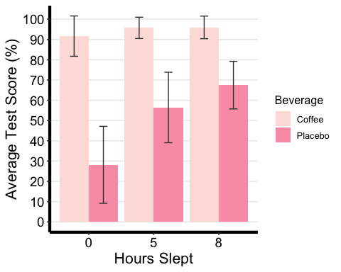
# Bar plot with two-factor variablesanova2w.barplot <-ggplot(mydata2w.summarystat, aes(x =factor(Sleep), y = mean, fill = Beverage) ) +geom_bar(stat = "identity", position = "dodge") +geom_errorbar(aes(ymax = mean + sd, ymin = mean - sd), #adding standard error barsposition =position_dodge(0.9), width = 0.25, color = "Gray25") +xlab("Hours Slept") +ylab("Average Test Score (%)") +scale_fill_brewer(palette = "RdPu") +theme_classic2() +theme(axis.line=element_line(linewidth=1.5), #thickness of x-axis lineaxis.text =element_text(size = 14, colour = "black"),axis.title =element_text(size = 16, colour = "black"),panel.grid.major.y =element_line() ) +# adding horizontal grid linesscale_y_continuous(breaks=seq(0, 100, 10)) # Ticks on y-axis from 0-100, # jumps by 10 anova2w.barplot
Computing the Repeated Measures Two-Way ANOVA
mydata2w.2anova <-anova_test(data = mydata2w,dv = TestScore, wid = ID, within =c(Beverage, Sleep), #for more than 2 factors to count you must use c()#it combines 2+ values into a vector/listdetailed = TRUE, effect.size = "ges"#we get the generalized eta squared, enter pes to get ) # partial eta squared# Apply the Greenhouse Geisser correction on an as-needed-basismydata2w.2anova <-get_anova_table(mydata2w.2anova, correction = "auto")
# We can calculate partial eta square and add it as a new column named "pes"mydata2w.2anova$pes = mydata2w.2anova$SSn/(mydata2w.2anova$SSn + mydata2w.2anova$SSd)
# Calculate the mean sum of error and add it as a new column named "MSE"mydata2w.2anova$MSE = mydata2w.2anova$SSd/mydata2w.2anova$DFd
# Convert tables to data framesmydata2w.2anova <-data.frame(mydata2w.2anova)
# Deleting intercept info (first row)mydata2w.2anova <- mydata2w.2anova[-1, ]
# Rename columnscolnames(mydata2w.2anova)[colnames(mydata2w.2anova) =="pes"] ="η2P"colnames(mydata2w.2anova)[colnames(mydata2w.2anova) =="ges"] ="η2G"colnames(mydata2w.2anova)[colnames(mydata2w.2anova) =="p..05"] ="sig"mydata2w.2anova
## Effect DFn DFd SSn SSd F p sig η2G η2P MSE
## 2 Beverage 1.00 85.00 246966.79 18527.547 1133.025 6.47e-51 * 0.752 0.930 217.9711
## 3 Sleep 1.34 113.78 44095.24 12457.452 300.872 8.82e-39 * 0.351 0.779 109.4872
## 4 Beverage:Sleep 1.60 136.23 27663.08 9544.342 246.362 2.23e-41 * 0.254. 0.743 70.0605
Any significant two-way interactions in this analysis must be followed up by further analyses looking at the effect of the other factor while keeping the level of another constant.
In these analyses, a significant two-way interaction indicates that the impact that one factor (e.g., Beverage) has on the outcome variable (e.g., test score) depends on the level of the other factor (e.g., Sleep) (and vice versa). So, you can decompose a significant two-way interaction by treating factor A to a one-factor ANOVA at each level of factor B.
Procedure for a significant two-way interaction:
Simple main effect: run a one-way model of one factor by keeping the level of the other constant. As in, run two one-way ANOVAs for one factor at each level of the other factor.
Simple pairwise comparisons: if the result of either of the one-way analyses is significant as in if the simple main effect is significant, then you will run multiple pairwise comparisons to determine which groups are different as we did previously for the one-way ANOVA tutorial.
# Simple Main Effect# Looking at the effect of Sleep separately for each level of Beverage mydata2w.one.way <- mydata2w %>%group_by(Beverage) %>%anova_test(dv = TestScore, wid = ID, within = Sleep) %>%get_anova_table() %>%adjust_pvalue(method = "bonferroni")mydata2w.one.way
## # A tibble: 2 × 9## Beverage Effect DFn DFd F p `p<.05` ges p.adj## <fct> <chr> <dbl> <dbl> <dbl> <dbl> <chr> <dbl> <dbl>## 1 Coffee Sleep 1.17 99.4 22.4 2.11e- 6 * 0.07 4.22e- 6## 2 Placebo Sleep 1.51 128. 331 1.76e-45 * 0.51 3.52e-45
There was a significant effect of sleep for both levels of the Beverage factor. We must now conduct pair-wise comparisons to determine where the difference in levels of sleep lies separately at both levels of beverage.
# Pairwise comparisons between Sleep levelsmydata2w.pwc <- mydata2w %>%group_by(Sleep) %>%pairwise_t_test( TestScore ~ Beverage, paired = TRUE,p.adjust.method = "bonferroni" )mydata2w.pwc
## # A tibble: 3 × 11
## Sleep .y. group1 group2 n1 n2 statistic df p p.adj p.adj.signif
## * <fct><chr><chr><chr> <int><int><dbl><dbl><dbl> <dbl><chr>
## 1 0 TestScore Coffee Placebo 86 86 35.1 85 2.32e-52 2.32e-52
## 2 5 TestScore Coffee Placebo 86 86 22.0 85 6.52e-37 6.52e-37
## 3 8 TestScore Coffee Placebo 86 86 25.7 85 8.84e-42 8.84e-42
Interpreting & Analyzing Results
The two-way repeated measures ANOVA revealed a significant main effect of beverage [F(1,85)= 1133.0, MSE = 218.0, partial eta squared = 0.930], and sleep [F(1.3,113.8)= 300.9, MSE = 109.5, partial eta squared = 0.780], qualified by a two-way interaction [F(1.6,136.2)= 300.9, MSE = 70.1, partial eta squared = 0.743]. Considering the Bonferroni adjusted p-value (p.adj), it can be seen that the simple main effect of sleep was significant at both levels of Beverage [Coffee, p<0.001; Placebo, p<0.001]. Pairwise comparisons show that the mean test score was significantly different between coffee and placebo conditions at 0 hours (p < 0.0001) and 5 hours (p < 0.0001) and 8 hours (p < 0.0001) of overnight sleep.
Note that instead of decomposing the sleep x beverage two-way interaction into the simple main effect of beverage, you could have chosen sleep. As in performing the same analysis for the sleep variable at each level of beverage, You don’t necessarily need to do this analysis. You simply have to interchange when the factors Sleep and Beverage are plugged into the codes for the post hoc analyses.
What if: Non-Significant Two-Way Interaction
Importantly, if the two-way interaction was not significant in the overall ANOVA, but there were still significant main effects (e.g., the main effect of Sleep and the main effect of Beverage), then you need to interpret the main effects for each of the two variables by conducting pairwise paired t-test comparisons.
# Comparisons for Beverage variable
mydata2w %>% pairwise_t_test( TestScore ~ Beverage, paired = TRUE, p.adjust.method = "bonferroni" )
# Comparisons for Sleep variable
mydata2w %>% pairwise_t_test( TestScore ~ Sleep, paired = TRUE, p.adjust.method = "bonferroni" )
Mixed Two-Way ANOVA
For practice, I encourage you to compute a mixed two-way ANOVA for the data file named "Practice_2WayANOVA_Mixed.xlsx" with the following elements:
- Measured Variable: TestScore
- 2 x 3 Mixed Design
- Between-Participants: "Exercise"
- Within-Participants: "Sleep"
In this hypothetical experiment, participants attended 3 lectures across different time points. One group of participants was asked to attend yoga classes three times a week for three months before the lecture series and attended yoga classes during the experiment. After one lecture session, they were asked to sleep for either 0 hours, 5 hours, or 8 hours before coming back the next day to be tested on the lecture. Another group of participants experienced a nearly identical experimental design, except that instead of yoga, they were asked to engage in mindfulness exercises.
We are interested in how sleep affects learning; in particular, whether test scores suffer when participants don't receive enough sleep. Moreover, we are also interested in whether those who engage in yoga are more resilient to this sleep-induced performance decrement. To the best of your ability visualize the data and compute the appropriate summary tables and figures to compare before going through the answers below.
# Data Prep & Summary Statisticsmydata2m <- read_excel("Practice_2WayANOVA_Mixed.xlsx")
mydata2m <- mydata2m %>% convert_as_factor(ID, Gender, Exercise, Sleep) str(mydata2m)
## tibble [516 × 7] (S3: tbl_df/tbl/data.frame)## $ ...1 : chr [1:516] "259" "260" "261" "262" ...## $ ID : Factor w/ 172 levels "23936","25440",..: 10 71 6 70 147 129 74 62 21 38 ...## $ Gender : Factor w/ 3 levels "F","M","Non-Binary": 1 1 1 1 1 1 1 3 1 2 ...## $ Age : num [1:516] 22 22 23 22 22 24 22 22 23 22 ...## $ Exercise : Factor w/ 2 levels "Mindfulness",..: 1 1 1 1 1 1 1 1 1 1 ...## $ Sleep : Factor w/ 3 levels "0","5","8": 1 1 1 1 1 1 1 1 1 1 ...## $ TestScore: num [1:516] 32 43 44 46 31 45 21 48 40 32 ...
mydata2m.summarystat <- mydata2m %>%group_by(Exercise, Sleep) %>%get_summary_stats(TestScore, type = "full")
# Selecting rows of data only if ID value is uniquemydata2m.unique <- mydata2m %>% distinct(mydata2m$ID, .keep_all=TRUE) # Looking at the distribution of "Gender" per grouptable(mydata2m.unique$Gender, mydata2m.unique$Exercise)
## Mindfulness Yoga
## F 40 60
## M 39 21
## Non-Binary 7 5
# Mean Age Per Group
mydata2m %>% group_by(Exercise) %>% get_summary_stats(Age, type ="mean")
## # A tibble: 2 × 4
## Exercise variable n mean
## <fct> <fct> <dbl> <dbl>
## 1 Mindfulness Age 258 22.6
## 2 Yoga Age 258 22.2
mydata2m.summarystat
## # A tibble: 6 × 15
## Exercise Sleep variable n min max median q1 q3 iqr mad mean sd se ci
## <fct> <fct> <fct> <dbl> <dbl> <dbl> <dbl> <dbl> <dbl> <dbl> <dbl> <dbl> <dbl> <dbl> <dbl>
## 1 Mindful… 0 TestSco… 86 15 48 32 23.2 41.8 18.5 13.3 32.3
## 2 Mindful… 5 TestSco… 86 38 80.8 48 43 53 10 7.41 48.7
## 3 Mindful… 8 TestSco… 86 55 66 59 57 63 6 4.45 60.1
## 4 Yoga 0 TestSco… 86 35 55 44.5 40.2 51 10.8 8.15 45.5
## 5 Yoga 5 TestSco… 86 66 80 72.5 68 76 8 6.67 72.7
## 6 Yoga 8 TestSco… 86 74 100 85.5 79 93.8 14.8 11.1 86.6
I will be skipping over the visualization step here since you can use the same codes as those for the within-subjects 2-way ANOVA here. I encourage you to practice making some summary plots on your own.
Computing the Two-Way ANOVA
mydata2m.2anova <- anova_test(data = mydata2m,dv = TestScore, wid = ID, between = Exercise, #between-participants factorwithin = Sleep, detailed = TRUE, effect.size = "ges" )# Apply the Greenhouse Geisser correction on an as-needed-basismydata2m.2anova <- get_anova_table(mydata2m.2anova, correction = "auto")# Calculate partial eta square and add it as a new column named "pes"mydata2m.2anova$pes = mydata2m.2anova$SSn/(mydata2m.2anova$SSn + mydata2m.2anova$SSd)# Calculate the mean sum of error and add it as a new column named "MSE"mydata2m.2anova$MSE = mydata2m.2anova$SSd/mydata2m.2anova$DFd# Convert tables to data framesmydata2m.2anova <- data.frame(mydata2m.2anova)# Deleting intercept info (first row)mydata2m.2anova <- mydata2m.2anova[-1, ]# Rename columnscolnames(mydata2m.2anova)[colnames(mydata2m.2anova) == "pes"] ="η2P" colnames(mydata2m.2anova)[colnames(mydata2m.2anova) == "ges"] ="η2G" colnames(mydata2m.2anova)[colnames(mydata2m.2anova) == "p..05"] ="sig"mydata2m.2anova
## Effect DFn DFd SSn SSd F p sig η2G η2P MSE
## 2 Exercise 1.00 170.0 57969.259 7475.35 1318.303 5.27e-82 * 0.699 0.8857759 43.97265
## 3 Sleep 1.89 321.9 104622.988 17468.35 1018.179 9.08e-137 * 0.807 0.8569239 54.26638
## 4 Exercise:Sleep 1.89 321.9 4365.807 17468.35 42.488 2.05e-16 * 0.149 0.1999531 54.26638
Procedure for a significant two-way interaction:
# Simple main effect of Exercise at each level of the Sleep factoranova2m.one.way <- mydata2m %>%group_by(Sleep) %>%anova_test(dv = TestScore, wid = ID, between = Exercise) %>%get_anova_table() %>%adjust_pvalue(method = "bonferroni")anova2m.one.way
## # A tibble: 3 × 9
## Sleep Effect DFn DFd F p `p<.05` ges p.adj
## <fct> <chr> <dbl> <dbl> <dbl> <dbl> <chr> <dbl> <dbl>
## 1 0 Exercise 1 170 109 4.39e-20 * 0.392 1.32e-19
## 2 5 Exercise 1 170 642 1.34e-59 * 0.791 4.02e-59
## 3 8 Exercise 1 170 742 6.34e-64 * 0.814 1.90e-63
OR you may opt to decompose the Exercise x Sleep interaction into the simple main effect of sleep for each exercise group (code included below); however since we are aware that test scores suffer when participants don't get enough sleep, this may not be sensible. Here we are more interested in whether yoga alleviates these sleep-induced performance decrements, therefore, we want to compare average test scores across the two groups when equating the amount of sleep. Therefore, you should give some thought to how you want to define your two-way interaction so that it addresses your research question.
# Simple main effect of Sleep for each Exercise Group # anova2m.one.way.alt <- mydata2m %>%# group_by(Exercise) %>%# anova_test(dv = TestScore, wid = ID, within = Sleep) %>%# get_anova_table() %>%# adjust_pvalue(method = "bonferroni")#anova2m.one.way.alt
Since the simple main effect of Exercise was significant, we must now run multiple pairwise comparisons to determine which groups are different.
# Pairwise comparisons between Exercise levelsanova2m.pwc <- mydata2m %>%group_by(Sleep) %>%pairwise_t_test(TestScore ~ Exercise, p.adjust.method = "bonferroni")anova2m.pwc
## # A tibble: 3 × 10## Sleep .y. group1 group2 n1 n2 p p.signif p.adj p.adj.signif## * <fct> <chr> <chr> <chr> <int> <int> <dbl> <chr> <dbl> <chr> ## 1 0 TestS… Mindf… Yoga 86 86 4.39e-20 **** 4.39e-20 **** ## 2 5 TestS… Mindf… Yoga 86 86 1.34e-59 **** 1.34e-59 **** ## 3 8 TestS… Mindf… Yoga 86 86 6.34e-64 **** 6.34e-64 ****
# If you computed the simple main effect of sleep the pairwise comparisons would be as such:#anova2m.pwc.alt <- mydata2m %>%# group_by(Exercise) %>%# pairwise_t_test(TestScore ~ Sleep, p.adjust.method = "bonferroni")#anova2m.pwc.alt
Interpreting & Reporting
EXAMPLE: The mixed two-way ANOVA revealed a significant main effect of exercise [F(1,170)= 1318.3, MSE = 44.0, partial eta squared = 0.886], and sleep [F(1.9,322)= 1018.2, MSE = 54.3, partial eta squared = 0.857], qualified by a two-way interaction [F(1.9,322)= 42.5, MSE = 54.3, partial eta squared = 0.120]. Considering the Bonferroni adjusted p-value (p.adj), it can be seen that the simple main effect of exercise was significant for all levels of the sleep factor [p<0.001].
Pairwise comparisons show that mean test score was significantly different between the two exercise groups across all levels of sleep, such that the yoga group scored higher on the test than the mindfulness group when participants slept for 0 hours (13.1%, p <0.0001), 5 hours (24.%, p <0.0001), or 8 hours (26.5%, p <0.0001) the night before the test (see Figure 1).
Note that here I am pointing my reader to a Figure (bar plot), so they can see that the Yoga group outperformed the mindfulness group. I’ve generated a bar plot for my Figure 1 here. I highly encourage you to recreate this plot (with standard error bars) or any other type of plot that summarizes the data well. Moreover, using the summary statistic table I’ve calculated the difference in average test scores for the appropriate comparisons.

