19 RStudio Workshop: One-Way ANOVA
Between-Subjects One-Way ANOVA
In our first hypothetical experiment, participants attended a lecture and were asked to come back the next day to take a test on the lecture material after having received either 0, 5, or 8 hours of sleep. Therefore, sleep is manipulated between participants. Here we are interested in the effect of hours slept on test scores, we can do this by conducting a one-way analysis of variance (ANOVA).
A one-way ANOVA is an extension of an independent two-sample t-test. Here, the data is organized into several groups of participants (e.g., 3 groups) based on a single grouping variable, also called a factor variable (e.g., sleep). You can think of a factor as an independent variable with more than 2 levels of manipulation. In our case, we have three different levels of manipulation to sleep.
Therefore, in a one-factor ANOVA, we are comparing means in a situation where there are more than two levels to a single factor. The aim of this tutorial is to describe the basic principle of the one-way ANOVA test and provide practical ANOVA test examples in R software.
NOTE: if you have only two groups, an F-test and a t-test are the same.
In an ANOVA we are testing two hypotheses: 1. Null hypothesis: there is no difference between the means of the different groups 2. Alternative hypothesis: there is a difference in means between at least two groups.
Now, we aim to reject the null hypothesis in favour of the alternative, by showing that there is a significant difference between at least 2 groups of participants.
The first step in doing so is to import our data set, then inspect our file.
# Now when it comes to importing your data frame I prefer to do so using the following code which allows me to click on my data frame, but you can also load your data frame by calling on the document's name.mydata1 <- read_excel(file.choose()) # If your data frame is in csv format use read.csv(file.choose())# or # if you already know the name of your data file and have set the working # directory, you can import you data file by namemydata1 =read_excel("OneWay_Sample_DataFile.xlsx") # or read.csv("OneWay_Sample_DataFile.csv")
# Let's inspect our data frameprint(mydata1) # look at the entire data frame
## # A tibble: 258 × 5## ID Gender Age Sleep TestScore## <chr> <chr> <dbl> <chr> <dbl>## 1 259 F 27 0 53.3## 2 260 F 22 0 66.0## 3 261 F 19 0 56.3## 4 262 F 25 0 68.7## 5 263 Non-Binary 23 0 77.4## 6 264 F 27 0 19.3## 7 265 F 30 0 31.1## 8 266 Non-Binary 27 0 64.5## 9 267 F 18 0 42.4## 10 268 M 28 0 32.9## # ℹ 248 more rows
# or you can use head(mydata1) #look at the first 6 rows
Note that in R studio, once you load your data file, you will notice it pop up under the name you saved it as, which in this case is “mydata1” at the top right corner of your screen, which is your global environment. Here you will see all your stored work, values, and files. You can click on the data file under data to open it as a separate tab beside your script, to look through, or you can do this exact action by code using view(). I tend to use this function when my global environment gets super packed, and it is no longer feasible to scan through the multitude of data for a specific one I want to take a look at.
view(mydata1) # to open the entire data file in a separate tab in R studio
Now in this data file, ID distinguishes between individual participants.
We also have some basic demographic info, including “Age” and “Gender”, which we typically summarize and report when describing our sample size in our Methods section. These demographic info may differ depending on your test subjects, but these are the typical ones we report with human subjects.
In this data file, our numerical dependent variable is in percentage form out of 100% (“TestScore”).
Our factor is in the column “Sleep”. Let’s check out to see if the factor is set up correctly by looking at the structure of our data frame.
str(mydata1) # looking at the structure of the data frame
## tibble [258 × 5] (S3: tbl_df/tbl/data.frame)## $ ID : chr [1:258] "259" "260" "261" "262" ...## $ Gender : chr [1:258] "F" "F" "F" "F" ...## $ Age : num [1:258] 27 22 19 25 23 27 30 27 18 28 ...## $ Sleep : chr [1:258] "0" "0" "0" "0" ...## $ TestScore: num [1:258] 53.3 66 56.3 68.7 77.4 ...
We can see that our dependent measure “TestScore” is set up correctly as numerical. If not, then we need to fix it by using the following code:
mydata1$TestScore <- sapply(mydata1$TestScore, as.numeric)
Note that by using “$” beside our data frame name, we are calling upon a column name, as you start typing you will notice that a list of all the column names comes up as a short-cut.
We can also see that ID and Sleep are not set-up as factors. Let’s fix that.
# Lets set up our factormydata1 <- mydata1 %>%convert_as_factor(ID, Sleep)
# Lets double-check to make sure that our factor is set-up correctly. levels(mydata1$Sleep)
## [1] "0" "5" "8"
Summary Statistics
Next, let’s compute some summary statistics for each group across the different levels of Sleep.
ANOVA1.summary.statistics <-data.frame (mydata1 %>%group_by(Sleep) %>%# enter factor(s)get_summary_stats(TestScore, type = "full") )
ANOVA1.summary.statistics
## Sleep variable n min max median q1 q3 iqr mad mean## 1 0 TestScore 86 6.860 93.301 45.687 29.348 59.249 29.901 23.390 45.873## 2 5 TestScore 86 34.117 93.301 74.726 62.563 83.734 21.171 16.138 71.696## 3 8 TestScore 86 47.587 93.301 85.748 77.358 90.314 12.956 7.858 82.526## sd se ci## 1 20.850 2.248 4.470## 2 15.570 1.679 3.338## 3 10.092 1.088 2.164
Here I am looking for group means along with the standard error of the mean values, which I will later use for my error bars when making figures. Some other measures that you can use are listed under the info card for the get_summary_stats function and include: type = c(“mean_sd”, “mean_se”, “mean_ci”, “median_iqr”, “median_mad”, “quantile”, “mean”, “median”, “min”, “max”)
For example, you may be interested in using mean standard deviation values for your error bars, in which case you can use “mean_sd”. You may also use “full” as your type to get all the measures!
Pro Tip: You can explore what each function offers with examples by putting a “?” right before the empty function, as shown below. It will open up the information sheet for the function on the Help tab to your bottom right on R studio. Try it!
?get_summary_stats()
Making Publishable Tables
Now, while this is a nice table if you want to include these summary statistics in your final thesis paper. We can do the following steps to generate nice printable summary tables!
# First let's maintain our unedited copy with the full values, which # we will call on when making our plots & figures and a separate copy that # we will edit to make the publishable table. ANOVA1.summarystat.publishable <- ANOVA1.summary.statistics
# We will begin by rounding numerical values in each column to 3 significant # figures, but you may choose to change this depending on your own preferenceANOVA1.summarystat.publishable$mean <-signif(ANOVA1.summarystat.publishable$mean,3) ANOVA1.summarystat.publishable$se <-signif(ANOVA1.summarystat.publishable$se,3)
# Selecting columns by name that we want to include in our final table by nameANOVA1.summarystat.publishable <-subset(ANOVA1.summarystat.publishable, select =c(Sleep, n, mean, se))
# Next we will change column names to make them nicer#colnames(T2.summary.statistics) # to print all column names in data frame if you don't remembercolnames(ANOVA1.summarystat.publishable)[colnames(ANOVA1.summarystat.publishable) =="n"] ="N"colnames(ANOVA1.summarystat.publishable)[colnames(ANOVA1.summarystat.publishable) =="mean"] ="Mean"colnames(ANOVA1.summarystat.publishable)[colnames(ANOVA1.summarystat.publishable) =="se"] ="Standard Error"
# Generating the Printable Summary Stat Table ANOVA1.summarystat.publishable %>%kbl(caption = "Summary Statistics") %>% # Title of the tablekable_classic(full_width = F, html_font = "Cambria", font_size = 10) %>% add_header_above(c(" " = 2, "Test Score (%)" = 2)) # adding header to columns in table by position. # E.g., for the first 2 columns we do not want a header so we leave empty space. # Over the last two column we specified the header name.

Reporting Demographic Info As I mentioned before, one of the first things we have to do when writing up our Methods is to report some basic information about our sample size. Let’s do that now!
# Computing average age by groupmydata1 %>%group_by(Sleep) %>%get_summary_stats(Age, type = "mean")
## # A tibble: 3 × 4## Sleep variable n mean## <fct> <fct> <dbl> <dbl>## 1 0 Age 86 23.7## 2 5 Age 86 24.0## 3 8 Age 86 24.0
Note that n represents the number of participants per group, meaning that in total, we have data from 258 participants. More importantly, we can see that the number of observations per condition is equal, therefore, this is a balanced design. If you have an unequal sample size, I recommend that you refer to the following link for more information on conducting an unbalanced ANOVA:
How to perform one-way anova with unequal sample sizes in R?
However, I would still recommend reading through this guide to become familiar with R-studio. You will be doing the same steps when doing an unbalanced ANOVA, with some adjustments to the code.
# Looking at the distribution of "Gender" across the three groupstable(mydata1$Gender, mydata1$Sleep) %>%#each cell represents the number of subjects in this categoryaddmargins() ## we can add margins to the table to make it clearer
## ## 0 5 8 Sum## F 37 36 45 118## M 39 40 33 112## Non-Binary 10 10 8 28## Sum 86 86 86 258
Reporting Participants
Here is an example of how you might report information about your sample size in your Methods section based on the above summary tables.
Example: We recruited 258 participants from the introductory psychology undergraduate participant pool at McMaster University in exchange for partial course credit. Participants were randomly assigned to either the no sleep condition (39 males and 10 non-binary; Mean age = 23.7 years), 5 hour sleep condition (n=86; 40 males and 10 non-binary; Mage = 24.0 years), or the 8 hour sleep condition (n=86; 33 males and 8 non-binary; Mage = 24.0 years)
Visualization: Generating Plots & Figures
With our summary statistics in hand. Let’s generate some nice summary plots to visualize our data!=
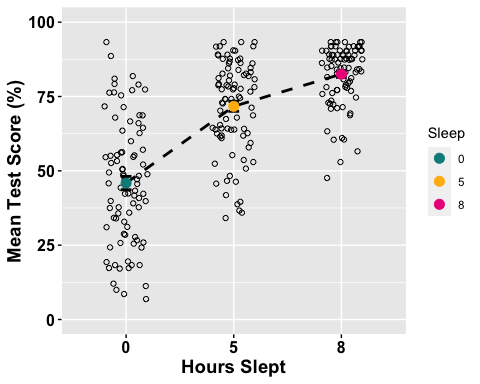
LINE PLOT
The first one we will create is a line plot. So here we want to specify which factor we want on our x-axis, as well as which summary measure of our dependent variable we want on our y-axis. In this case, we want the Sleep factor (with 3 levels) on the x-axis, and mean Test Scores on the y-axis
Tip: One thing to keep in mind is that you should design your plots such that if a reader is colour-blind or chooses to print your results in black-white, they can still easily distinguish between the different factors in your plot. Hence, we will also use the shape of our points to also specify “BLOCK_TYPE”
anova1.lineplot <-ggline(mydata1, x = "Sleep", y = "TestScore",add =c("mean_se", "jitter"), #adding standard error bars and jitter # points representing each individual participant in each group. order =c("0", "5", "8"), #organizing order of levelsylab = "Mean Test Score (%)", xlab = "Hours Slept", #adding x- and y-axis title color = "black", #colour of linelinetype = "dashed", font.label =list(size = 20, color = "black"),size = 1,point.color = "Sleep", #point color differs for each level of the Sleep factorpalette =c("cyan4", "darkgoldenrod1", "deeppink2"),shapes = 1, #point shapespoint.size = 2,ggtheme =theme_gray(),ylim=c(0,100) #adjusting the min and max value of y-aixs )# For more options run the ?ggline() code# Change the appearance of titles and labelsanova1.lineplot +font("xlab", size = 14, color = "black", face = "bold")+font("ylab", size = 14, color = "black", face = "bold")+font("xy.text", size = 12, color = "black", face = "bold")
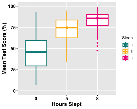
BOX PLOT
anova1.boxplot <-ggboxplot(mydata1, x = "Sleep", y = "TestScore", color = "Sleep", palette =c("cyan4", "darkgoldenrod1", "deeppink2"), order =c("0", "5", "8"),ylab = "Mean Test Score (%)", xlab = "Hours Slept",add = ("median_iqr"), #adding median and inner quartile rangefont.label =list(size = 20, color = "black"),size = 1,ggtheme =theme_gray(),ylim=c(0,100) #adjusting the min and max value of y-aixs )
# Change the appearance of titles and labelsanova1.boxplot +font("xlab", size = 14, color = "black", face = "bold")+font("ylab", size = 14, color = "black", face = "bold")+font("xy.text", size = 12, color = "black", face = "bold")
# For more options run the ?ggboxplot() code
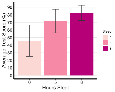
BAR PLOT
If you are interested in exploring your options when it comes to bar plots, I recommend the following resources:
- Step-by-Step Barplots for One Factor in R
- ggplot2 barplots : Quick Start Guide
- This post explains how to draw barplots with R and ggplot2, using the geom_bar() function.
- Elegant barplot using ggplot function in R
The following link will show you all the different colour palettes that you can use for designing plots.
# Notice that I am using the summary statistic table with the full range of # summary data not the printable one we made. anova1.barplot <-ggplot(ANOVA1.summary.statistics, aes(x =factor(Sleep), y = mean, fill = Sleep) ) +geom_bar(stat = "identity", position = "dodge") +geom_errorbar(aes(ymax = mean + sd, ymin = mean - sd), #adding standard error barsposition =position_dodge(0.9), width = 0.25, color = "Gray25") +xlab("Hours Slept") +ylab("Average Test Score (%)") +scale_fill_brewer(palette = "RdPu") +theme_classic() +theme(axis.line=element_line(linewidth=1.5), #thickness of x-axis lineaxis.text =element_text(size = 14, colour = "black"),axis.title =element_text(size = 16, colour = "black"),panel.grid.major.y =element_line() ) +# adding horizontal grid linesscale_y_continuous(breaks=seq(0, 100, 10)) # Ticks on y-axis from 0-100, # jumps by 10 anova1.barplot
Computing a One-Way ANOVA
# Computing the one-way ANOVAone.aov <-aov(TestScore ~ Sleep, data = mydata1)# Summary of the analysissummary(one.aov)
## Df Sum Sq Mean Sq F value Pr(>F) ## Sleep 2 60991 30496 117.4 <2e-16 ***## Residuals 255 66212 260 ## ---## Signif. codes: 0 '***' 0.001 '**' 0.01 '*' 0.05 '.' 0.1 ' ' 1
Interpreting & Reporting
We can see that the p-value (Pr(>F)) is significantly less than the significance level of 0.05, as highlighted by the “asterisk” symbols in the summary table. Therefore we can reject the null hypothesis that there were no differences between groups. When reporting these data, we typically have to report the degrees of freedom, the F value, p-value, and a measure of effect size). Next we are going to calculate effect sizes, in specific, we will be reporting partial eta squared here. You should consult with your principal investigator on which measure of effect size they deem appropriate.
For a more comprehensive review of the effect size measure options please go to the following resource: Effect Sizes for ANOVAs
options(es.use_symbols = TRUE) # get nice symbols when printing! (On Windows, requires R >= 4.2.0)eta_squared(one.aov, partial = TRUE)
## For one-way between-subjects designs, partial eta squared is equivalent to eta squared. Returning eta squared.
## # Effect Size for ANOVA## ## Parameter | η² | 95% CI## -------------------------------## Sleep | 0.48 | [0.41, 1.00]## ## - One-sided CIs: upper bound fixed at [1.00].
Pair-Wise Comparisons
Next, while our one-way ANOVA showed that there is a significant difference between groups, we don’t know which pairs of groups are different. Using multiple pairwise comparisons, we can probe where this difference lies between pairs of groups.
In R, there are multiple functions for conducting the same analyses. My personal favourite for this next step is the function TukeyHD(), which takes our fitted one-way ANOVA as an argument.
TukeyHSD(one.aov, conf.level = 0.95#you may change this, default is 0.95)
## Tukey multiple comparisons of means## 95% family-wise confidence level## ## Fit: aov(formula = TestScore ~ Sleep, data = mydata1)## ## $Sleep## diff lwr upr p adj## 5-0 25.82300 20.029891 31.61610 0.00e+00## 8-0 36.65349 30.860383 42.44659 0.00e+00## 8-5 10.83049 5.037386 16.62360 4.58e-05
When interpreting this output:
- diff: the difference between the means of the two groups
- lwr and upr correspond to the lower and the upper-end point of the confidence interval at 95%.
- p adj: p-value after adjustment for the multiple comparisons
It can be seen from the output that there is a significant difference between all combinations of the groups! However, the biggest benefit in performance occurs when participants receive 8 hours of sleep compared to no sleep.
Together with our ANOVA summary table, we now have everything we need to report our results.
Reporting Results:
The test score was statistically significantly different at the different amounts of sleep [F(2, 255) = 117.4, p < 0.001, pη² = 0.48]. Post-hoc analyses with a Bonferroni adjustment revealed that all the pairwise differences, between sleep levels, were statistically significantly different (p < 0.001).
Repeated Measures One-Way ANOVA
In the first experiment, we computed a one-way ANOVA for a factor that was manipulated between subjects, Meaning that we compared different groups to one another. Let’s compute a within-participants ANOVA.
In this hypothetical experiment, a group of participants are tested at three different time points, and most importantly, they all experience different sleep manipulations.
mydata1within <- read_excel("OneWayWithin_Sample_DataFile.xlsx")
# Set-up factormydata1within <- mydata1within %>%convert_as_factor(ID, Sleep)str(mydata1within) #checking data structure and how factor is set-up
## tibble [258 × 5] (S3: tbl_df/tbl/data.frame)## $ ID : Factor w/ 86 levels "29057","32239",..: 20 48 84 61 22 23 25 29 72 69 ...## $ Gender : chr [1:258] "F" "M" "F" "F" ...## $ Age : num [1:258] 23 22 23 23 22 22 22 22 22 22 ...## $ Sleep : Factor w/ 3 levels "0","5","8": 1 1 1 1 1 1 1 1 1 1 ...## $ TestScore: num [1:258] 45.77 17.56 16.6 49.59 8.51 ...
Summary Statistics
mydata1within %>%group_by(Sleep) %>%get_summary_stats(TestScore, type = "mean_se")
## # A tibble: 3 × 5## Sleep variable n mean se## <fct> <fct> <dbl> <dbl> <dbl>## 1 0 TestScore 86 30.8 2.43## 2 5 TestScore 86 56.4 1.88## 3 8 TestScore 86 67.5 1.26
I will be skipping over some of the steps, such as summarizing demographic info and visualizing the data. But you can use the same codes as those for the between-one-way ANOVA for this one. The main difference lies in computing the actual ANOVA, where we will be using a different function.
Computing Repeated Measures One-Way ANOVA
one.aov.within <- anova_test(data = mydata1within, #data frame dv = TestScore, #(numeric) dependent variable namewid = ID, #subjects identifier; must be unique per participantwithin = Sleep, # within-subjects factor variableseffect.size = "pes", #default is generalized eta square "ges" but here we specify that we want partial eta squared detailed = TRUE, #If TRUE, returns extra information (such as sums of squares columns, intercept row, etc.) in the ANOVA table )# Run ?anova_test() to explore more options for this function.
get_anova_table(one.aov.within, correction = "auto") #automatically apply GG correction to only within-subjects factors violating the sphericity assumption
## ANOVA Table (type III tests)## ## Effect DFn DFd SSn SSd F p p<.05 pes## 1 (Intercept) 1.00 85.00 686279.36 59317.41 983.417 1.71e-48 * 0.92## 2 Sleep 1.37 116.22 60840.19 21389.16 241.777 2.37e-35 * 0.74
From the ANOVA table, we can see that there was a significant effect of sleep on test scores. Next we want to see where the differences in scores lies.
Post-Hoc Analyses
one.anova.within.pwc <- mydata1within %>%pairwise_t_test( TestScore ~ Sleep, paired = TRUE,p.adjust.method = "bonferroni" )one.anova.within.pwc
## # A tibble: 3 × 10## .y. group1 group2 n1 n2 statistic df p p.adj p.adj.signif## * <chr> <chr> <chr> <int> <int> <dbl> <dbl> <dbl> <dbl> <chr> ## 1 Test… 0 5 86 86 -14.7 85 5.39e-25 1.62e-24 **** ## 2 Test… 0 8 86 86 -17.1 85 2.69e-29 8.07e-29 **** ## 3 Test… 5 8 86 86 -10.3 85 1.15e-16 3.45e-16 ****
